Regular Article
Investigation on the pressure response behavior of two-layer vertical mixed boundary reservoir: field cases in Western Sichuan XC gas field, China
1
State Key Laboratory of Petroleum Resources and Prospecting, China University of Petroleum, 102249 Beijing, PR China
2
University of Leeds, LS2 9JT Leeds, UK
3
SINOPEC Petroleum Exploration and Production Research Institute, 100083 Beijing, PR China
* Corresponding authors: This email address is being protected from spambots. You need JavaScript enabled to view it.
; This email address is being protected from spambots. You need JavaScript enabled to view it.
Received:
23
June
2020
Accepted:
15
October
2020
Abstract
Pressure response behavior of two-layered reservoir with a vertical mixed boundary is easy to be mistaken for that of the radial composite reservoir or dual-pore reservoir. It is difficult to fit the pressure response curve and easy to obtain abnormal parameter values using a misunderstood model. In this paper, we present the interpretation of three different types of pressure responses of vertical mixed boundary reservoir by our proposed models, where the diagnostic window and feature value are captured for different mixed boundary types. Results show that the mixed boundary with closed boundary and infinite-acting boundary induces the fake pressure response of a radial composite reservoir with poor permeability outer zone. The mixed boundary with the main constant-pressure and non-main closed boundary produces a fake pressure response of a dual-porosity reservoir. The diagnostic window of pressure response curves shape can easily capture the mixed boundary type, and the feature value of the feature values of pressure response value can quickly obtain the permeability ration of one layer. Aiming at different representative types of pressure response cases in the western Sichuan XC gas field, China, we innovatively analyze them from a different perspective and get a new understanding of pressure response behavior of vertical mixed boundary, which provides a guideline for the interpretation of layered oil and gas reservoir with the complex boundary in the vertical direction.
© W. Shi et al., published by IFP Energies nouvelles, 2020
 This is an Open Access article distributed under the terms of the Creative Commons Attribution License (https://creativecommons.org/licenses/by/4.0), which permits unrestricted use, distribution, and reproduction in any medium, provided the original work is properly cited.
Nomenclature
Parameters and variablesB: Fluid isotherm volume factor, m3/m3
C: Wellbore storage coefficient, m3/MPa
c: Fluid compressibility, MPa−1
c t : Total compressibility of the reservoir, MPa−1
h: Reservoir thickness of, m
k: Permeability, mD
p i : Initial reservoir pressure, MPa
p w : Bottom-hole pressure, MPa
q: Producing rate, m3/d
r: Radial distance, m
r e : Boundary distance, m
r w : Well radius, m
S: Skin factor, dimensionless
t: Production time, h
Z: Gas compressibility factor, dimensionless
μ: Viscosity, mPa·s
ϕ: Porosity, %
Subscripts and superscripts
 : Laplace domain parameter *
* D : Dimensionless parameter *
* j : Layer j Parameter *
* g : Gas parameter *
Symbols
∞: Infinite-acting boundary
Θ: Closed boundary
Ω: Const-pressure bounded boundary
1 Introduction
Modern well testing interpretation and analysis methods have a wide range of applications in acquiring reservoir physical property parameters and detecting reservoir boundary information [1–5]. Lefkovits et al. [6] first analyzed the pressure dynamic characteristics of combined production wells and laid the foundation for the well testing method of multi-layer combined production reservoirs. However, more and more oil and gas field reservoirs with complex boundaries have been discovered with the depletion of conventional oil and gas resources and the improvement of exploration technology.
The Pressure Transient Analysis (PTA) method is an effective technology to capture the boundary information of the layered reservoir based on the well test data [7]. Chao et al. [8] analyzed the responses of commingled systems with mixed inner and outer boundary conditions using pressure response derivatives and discussed the pressure response derivative characteristics of a unique reservoir radius in a two-layer reservoir. However, the two-layer reservoir only can capture the four type boundaries: the top-boundary distant larger than the bottom-boundary with high-permeability or low-permeability top-layer, and the bottom-layer distant larger than the top-layer with high-permeability or low-permeability top-layer. Shi et al. [9] extended the n-layered reservoir with the outer-convex shape reservoir boundary radius. Their case studies show that the pressure response of a reservoir with a vertical non-uniform boundary distance can easily be mistaken for the pressure response of a radial composite reservoir. Sun et al. [10] have proved that the vertical inhomogeneous closed boundary may produce a fake pressure response behavior of a radial composite reservoir with poor permeability outer zone, and interpreted this phenomenon by a type gas well in the western Sichuan Basin. Shi et al. [11] use a two-layer reservoir with different boundary types in the vertical direction show that the pressure response behavior in the radial composite reservoir model probably induced by a two-layer reservoir with one closed bounded layer and another infinite layer, and the pressure response behavior in dual-pore reservoir model may be caused by a two-layer reservoir with one closed layer and another constant-pressure layer.
Apart from using transient well testing pressure data, geophysical 4D seismic data is nowadays an important way to investigate boundaries [12]. Yin et al. [13] comprehensively reviewed the role of 4D time-lapse seismic technology as a reservoir monitoring and surveillance tool, and details discussed the application of 4D seismic technology in extending the life of hydrocarbon fields and improving hydrocarbon recovery, with specific consideration to the progresses made over the last decades. Suleen et al. [14, 15] applied the pressure transient analysis and 4D seismic to integrated waterflood surveillance. In their paper, the deep-water case study results show that the Integration of an engineering technique, namely PTA, with geophysical data such as 4D interpretation, lends deeper insights into the dynamic changes in the reservoir whereas either standalone method would be more limited in application. Yin et al. [16] enhanced the dynamic reservoir interpretation by correlating multiple 4D seismic monitors to well behavior. In detail, the cross-correlation, “well2seis”, was achieved by defining a linear relationship between the 4D seismic signals and changes in the cumulative fluid volumes at the wells. Sambo et al. [17] extended the newly developed “well2seis” technique to evaluate the inter-well connectivity using well fluctuations and 4D seismic data.
The XC gas field in western Sichuan, China, has developed abundant reverse faults in the northeast-southwest direction (Fig. 1a). The industrial production gas well is located near the fault zone because there are more high-angle cracks and fracture networks near the fault (Fig. 1b). The complex reservoir structure and fluid distribution bring many difficulties and challenges to capture the reservoir information and analyze the transient behavior of production gas well. Given the poor matching of the pressure response and abnormal parameter values of the XC gas field interpreted by the conventional radial composite reservoir and the dual-pore reservoir model, the results interpreted based on these misleading pressure response behaviors are likely to be wrong.
 |
Fig. 1 (a) Tectonic map of XC gas field. (b) Reservoir profile of XC gas field. |
To solve this problem and better understand this misleading pressure response phenomenon, this paper, based on the theoretical research of reference [11], reviews and extends three representative pressure responses behavior of the vertical mixed boundary reservoir. Firstly, the pressure response behavior and flow regime characteristics are summary and comparison under three mixed boundary types, including infinite mixed boundary, equidistant mixed boundary, and non-equidistant mixed boundary. After that, the diagnosis and capture method of three mixed boundary types is presented. Lastly, pressure responses of three typical production gas well in the XC gas field, Western Sichuan Basin, are interpreted by the models we proposed to give the transient pressure well-testing engineer and analyzer a new and comprehensive understanding of the pressure response behaviors in the vertical mixed boundary reservoir.
2 Methodology
2.1 Model and solution
The physical model of the two-layer mixed boundary reservoir with different boundary types and boundary distances as shown in Figure 2a. The basic assumptions are presented as follows:
-
The physical properties of each layer are different, including permeability (k), porosity (ϕ), total compressibility (c t ), thickness (h), pressure (p), boundary radius (r e ), boundary type (constant-pressure boundary Ω, closed boundary Θ, infinite-acting boundary ∞), and each horizontal layer is homogeneous isothermal and isotropic.
-
Before well opening, the reservoir is filled with single-phase, slightly compressible liquid. During production, the viscosity (μ) and volume factor (B) of liquid remain constant.
-
The initial pressure (p i ) in the upper layer and bottom layer are uniform before well opening. The well located at the center of the reservoir, and the bottom-hole pressure (p w ) changes with the production time when the production rate (q) is constant.
-
Fluid from each layer only flows radially into the wellbore (r w ) from that layer (Fig. 2b). No formation crossflow occurs between the upper layer and the bottom layer due to the existence of an impermeable interlayer (Fig. 2c).
-
The wellbore storage and skin effect are considered. The gravity effect and temperature change are negligible.
 |
Fig. 2 Physical model of two-layer mixed boundary reservoir. (a) Reservoir model. (b) Radial flow model. (c) Vertical flow model. |
Appendix A in reference [11] gives the dimensionless mathematical model of Figure 2 in the Laplace domain through the Laplace transform [18–20]. Based on the Bessel equation solution [21], Cramer’s rule [22], Duhamel’s principle [23], and Stehfest numerical inversion [24], Appendix B in reference [11] provides the dimensionless bottom-hole pressure response solution in the real-time domain. The pressure response and its derivative combined type curves in the log–log coordinate can be drawn to diagnose the flow characteristics and capture the boundary information. Appendix C in reference [11] provides the relationship between the draw-off well test method and the build-up well test method [25].
2.2 Pressure response behavior
2.2.1 Infinite mixed boundary
Figure 3 is the pressure and pressure derivative combined type curves of the mixed boundary reservoir with one layer bounded and other infinite. Table 1 is the flow regimes characteristics and pressure response behavior of Figure 3. where the pseudo-IARF is the identifiable feature in the identifiable window of the r eD [Θ] & r eD [∞], and “pseudo-CpBF” is the identifiable feature in the identifiable window of the r eD [Ω] & r eD [∞]. Readers should be careful to note that the pressure response behavior of r eD [Θ] & r eD [∞] is very similar to that of the radial composite reservoir with poor permeability outer zone.
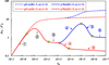 |
Fig. 3 Pressure response of infinite mixed boundary reservoir (two layers, one layer bounded and other infinite). (C D = 10, S = 3, κ[Ω] = κ[Θ] = 0.5, ω[Ω] = ω[Θ] = 0.5, r eD [Ω] = r eD [Θ] = 5000). |
2.2.2 Equidistant mixed boundary
Figure 4 is the pressure response behavior of the equidistant mixed boundary reservoir with one layer closed and other constant pressure. Table 2 is the boundary flow characteristics and pressure response behavior of Figure 4. The “first CBF and then CpBF” is the identification window of the r eD [Ω] = r eD [Θ]. The appearance of CBF means the closed layer is the main-flow layer (κ[Θ] > κ[Ω]), and the appearance of CpBF means the constant-pressure layer is the main-flow layer (κ[Ω] > κ[Θ]). Readers should be careful to note that the pressure response behavior of r eD [Ω] & r eD [Θ] when κ[Ω] > κ[Θ] is very similar to that of the dual-pores reservoir with an obvious V shape.
 |
Fig. 4 Pressure response of equidistant mixed boundary reservoir (two layers, one layer closed and other const-pressure). (C D = 10, S = 3, κ[Ω] ≠ κ[Θ], ω[Ω] = ω[Θ] = 0.5, r eD [Ω] = r eD [Θ] = 5000). |
2.2.3 Non-equidistant mixed boundary
Figure 5 is the pressure response behavior of the non-equidistant mixed boundary reservoir with the closed boundary closer than constant-pressure boundary (r eD [Θ] < r eD [Ω]). Table 3 is the boundary flow characteristics of Figure 5. The identification window of r eD [Θ] < r eD [Ω] is the first identifiable window of r eD [Θ] & r eD [∞] and then the identifiable window of r eD [Ω]. The larger the permeability ratio of closed layer k[Θ], the more obvious the identifiable window of r eD [Θ] & r eD [∞].
 |
Fig. 5 Pressure response of non-equidistant mixed boundary reservoir (closed boundary is near, and const-pressure boundary is far). (C D = 10, S = 3, κ[Θ] = {0.1, 0.9}, κ[Ω] = {0.1, 0.9}, ω[Ω] = ω[Θ] = 0.5, r eD [Θ] = 5000, r eD [Ω] = 500 000). |
Figure 6 is the pressure response behavior of the non-equidistant mixed boundary reservoir with the constant-pressure closer than closed boundary (r eD [Ω] < r eD [Θ]). Table 4 is the boundary flow characteristics of Figure 6. The identification window of r eD [Ω] < r eD [Θ] is the first identifiable window of r eD [Ω] & r eD [∞] and then the identifiable window of r eD [Ω] = r eD [Θ]. The larger the permeability ratio of constant-pressure layer k[Ω], the more obvious the identifiable window of r eD [Ω] & r eD [∞].
 |
Fig. 6 Pressure response of non-equidistant mixed boundary reservoir (const-pressure boundary is near, and closed boundary is far). (C D = 10, S = 3, κ[Θ] = {0.1, 0.9}, κ[Ω] = {0.1, 0.9}, ω[Ω] = ω[Θ] = 0.5, r eD [Ω] = 5000, r eD [Θ] = 500 000). |
3 Field cases
In this part, the well cases from the XC gas field, western Sichuan Basin, China are analyzed in detail through the models and methods provided above. As shown in Figure 1a, there are abundant reverse faults in the reservoir of the XC gas field in the North–South direction, and the overall reservoir is low in the east and high in the west. Figure 1b is the cross-well profile (X10–X301–X2–L150–X5–X601–CH127) of the blue line in Figure 1a. On the one hand, the cross-well profile shows the gas reservoir has obvious layered characteristics in the vertical direction. The upper layer is a low-porosity gas-bearing layer, the middle layer is a high-porosity gas-bearing layer, and the bottom layer is a water-bearing gas layer that gradually thins and disappears from east to west. On the other hand, there are a lot of cracks and fractures near the fault. Therefore, the reservoir is very complex and strongly heterogeneous in the vertical and horizontal directions. In the following analysis case, the reservoir of the target well stratified by the workflow shown in Figure 7. The workflow considers two judgment conditions, flow unit obtained by the logging data, and the geological unit came from the lithology profile and sedimentary facies. The method of judging the flow unit of a multi-layer reservoir can be found in reference [11].
 |
Fig. 7 Stratified workflow base on the logging data and geological information. |
3.1 Case well of closed and infinite model
Well#X10 is a vertical production gas well located in the Northeast corner of a northeast closed intersecting fault zone (Fig. 8e). In terms of flow unit, the pressure conductivity ratio distribution (Fig. 8d) is calculated by the logging date including the porosity (Fig. 8a), permeability (Fig. 8b), and thickness information (Fig. 8c). In terms of geological unit, the reservoir lithology profile (Fig. 8f) is yielded by the structure sedimentary facies (Fig. 8e). On the one hand, the flow unit and geological unit consistently show that the top zone (A in Fig. 8g) is a better production gas layer than the bottom zone (B in Fig. 8g). On the other hand, the top near-well zone is a relatively closed bounded zone due to there are a high-porous fracture network and fault (F1 in Fig. 8g) in the top far-well zone, and the bottom zone is a very wide water-bearing gas layer far larger than the top zone. Therefore, the mixed boundary reservoir model with bounded closed top zone and infinite-acting bottom zone, r eD [Θ] & r eD [∞], is used to analyze X10. The basic parameters including the reservoir parameters, gas parameters, and production parameters of X10 are listed in Table 5.
 |
Fig. 8 Basis and results of the stratified workflow of X10. (a) Porosity distribution of X10. (b) Permeability distribution of X10. (c) Thickness distribution of X10. (d) Pressure conductivity ratio distribution of X10. (e) Sedimentary structure map of X10. (f) Lithology profile of X10. (g) Reservoir stratification result of X10. |
Basic parameters of Well#X10.
Based on the relationship between the pressure draw-down and the pressure build-up, use the selected model r eD [Θ] & r eD [∞], to fit pressure build-up data of X10. The fitting curves as shown in Figure 9 and the reservoir and boundary information obtained by the fitting well test data as listed in Table 6. On the one hand, based on the empirical formula (see Tab. 1), the permeability ratio of the infinite-acting layer can be obtained by the pressure derivative value in Figure 9. In the log–log coordinate system, the empirical formula κ[∞] = l 0/l can be rewritten:
![Mathematical equation: $$ \kappa \left[\infty \right]={10}^{\frac{h}{H}}={10}^{\frac{0.95\enspace \mathrm{cm}}{1.83\enspace \mathrm{cm}}}=0.303. $$](/articles/ogst/full_html/2021/01/ogst200189/ogst200189-eq2.gif)
 |
Fig. 9 Well test data of X10 and fitting curves of model r eD [Θ] & r eD [∞]. |
Interpretation parameters of X10.
On the other hand, based on the definition of permeability ratio, the permeability ratio of the closed top zone can be quickly calculated by the value in Table 6:
![Mathematical equation: $$ \kappa \left[\mathrm{\Theta }\right]=\frac{k[\mathrm{\Theta }]h[\mathrm{\Theta }]}{k\left[\mathrm{\Theta }\right]\mathrm{h}\left[\mathrm{\Theta }\right]+k\left[\mathrm{\infty }\right]h[\mathrm{\infty }]}=\frac{0.23\enspace \mathrm{mD}\times 13.89\mathrm{\enspace }\mathrm{m}}{0.23\enspace \mathrm{mD}\times 13.89\enspace \mathrm{m}+0.03\enspace \mathrm{mD}\times 42.71\enspace \mathrm{m}}=0.714. $$](/articles/ogst/full_html/2021/01/ogst200189/ogst200189-eq3.gif)
3.2 Case well of constant-pressure and infinite model
Well#X3 is a vertical production gas well located in the east of north-south open and east-west closed zone. (see Fig. 10e). In terms of the flow unit, the reservoir pressure conductivity ratio (Fig. 10d) can be obtained by the logging data (Figs. 10a–10c). In terms of geological unit, the reservoir lithology profile (Fig. 10g) is yielded by the structure sedimentary facies (Fig. 10e) and imaging logging of adjacent well (Fig. 10f). On the one hand, the flow unit and geological unit consistently show that the top zone (A in Fig. 10h) is a better production gas layer than the bottom zone (B in Fig. 10h) due to there are abundant fractures network and high-angle cracks near the faults. On the other hand, the top near-well zone is a relatively stable pressure supply zone due to the high-angle cracks and faults connect the wide bottom pressure body (F1, F3, F4 in Fig. 10h). Therefore, the mixed boundary reservoir model with bounded constant-pressure top zone and infinite-acting bottom zone, r eD [Ω] & r eD [∞], is used to analyze X3. The basic parameters including the reservoir parameters, gas parameters, and production parameters of X3 are listed in Table 7.
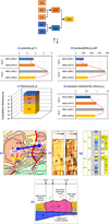 |
Fig. 10 Basis and results of the stratified workflow of X3. (a) Porosity distribution. (b) Permeability distribution. (c) Thickness distribution. (d) Pressure conductivity ratio distribution. (e) Sedimentary structure map of X3. (f) Imaging logging of X3. (g) Lithology profile of adjacent wells X301. (h) Reservoir stratification result of X301. |
Basic parameters of X3.
Based on the relationship between the pressure draw-down and the pressure build-up, use the selected model r eD [Ω] & r eD [∞], to fit pressure build-up data of X3. The fitting curves as shown in Figure 11 and the reservoir and boundary information obtained by the fitting well test data as listed in Table 8. On the one hand, based on the empirical formula (see Tab. 1), the permeability ratio of constant-pressure bottom zone can be obtained by the pressure derivative value in Figure 11:
![Mathematical equation: $$ \kappa \left[\mathrm{\Omega }\right]=\frac{m}{a}=\frac{\mathrm{tan}{\theta }_2}{\mathrm{tan}{\theta }_1}=\frac{0.307}{0.845}=0.365. $$](/articles/ogst/full_html/2021/01/ogst200189/ogst200189-eq4.gif)
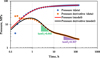 |
Fig. 11 Well test data of X3 and fitting curves of model r eD [Ω] & r eD [∞]. |
Interpretation parameters of X3.
On the other hand, based on the definition of permeability ratio, the permeability ratio of constant-pressure bottom zone can be quickly calculated by the value in Table 8:
![Mathematical equation: $$ \kappa \left[\mathrm{\Omega }\right]=\frac{k\left[\mathrm{\Omega }\right]h[\mathrm{\Omega }]}{k\left[\mathrm{\Omega }\right]h\left[\mathrm{\Omega }\right]+k\left[\mathrm{\infty }\right]h[\mathrm{\infty }]}=\frac{0.414\enspace \mathrm{mD}\times 8.5\enspace \mathrm{m}}{0.414\enspace \mathrm{mD}\times 8.5\enspace \mathrm{m}+0.198\enspace \mathrm{mD}\times 27\enspace \mathrm{m}}=0.397. $$](/articles/ogst/full_html/2021/01/ogst200189/ogst200189-eq5.gif)
3.3 Case well of closed and constant-pressure model
Well#X5 is a vertical production gas well located in the south of a groove-shaped closed fault zone (see Fig. 12e). In terms of the flow unit, the reservoir pressure conductivity ratio (Fig. 12d) can be obtained by the logging data (Figs. 12a–12c). In terms of the geological unit, reservoir lithology profile (Fig. 10g) is yielded by the structure sedimentary facies (Fig. 10e) and imaging logging (Fig. 10f). On the one hand, the flow unit and geological unit consistently show that the top zone (B in Fig. 12h) is a better production gas layer than the bottom zone (A in Fig. 12h) due to the porosity and permeability of the top zone is higher than that of the bottom zone. On the other hand, the imaging logging and reservoir profile consistently show the bottom water can easily invade the top zone through the fault (F4 & F5 in Fig. 12h) and high-angle cracks. Therefore, the mixed boundary reservoir model with bounded constant-pressure top zone and the bounded closed bottom zone, r eD [Ω] & r eD [Θ], is used to analyze X5. The basic parameters including the reservoir parameters, gas parameters, and production parameters of X5 are listed in Table 9.
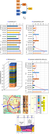 |
Fig. 12 Basis and results of the stratified workflow of X5. (a) Porosity distribution of X5. (b) Permeability distribution of X5. (c) Thickness distribution of X5. (d) Pressure conductivity ratio distribution of X5. (e) Sedimentary facies map of X5. (f) Imaging logging of X5. (g) Lithology profile of X5. (h) Reservoir stratification result of X5. |
Basic parameters of X5.
Due to the production time is far longer than the shut-in time, so the pressure draw-down response model chosen to fit the well test data. The fitting curves as shown in Figure 13 and the reservoir and boundary information obtained by the fitting well test data as shown in Table 10. On the one hand, based on the empirical formula (see Tab. 2), the permeability ratio of constant-pressure layer can be obtained by the pressure value in Figure 13:
![Mathematical equation: $$ \kappa \left[\mathrm{\Omega }\right]=\frac{{L}_0}{L}=\frac{14.80}{17.22}=0.859. $$](/articles/ogst/full_html/2021/01/ogst200189/ogst200189-eq6.gif)
 |
Fig. 13 Well test data of X5 and fitting curves of model r eD [Ω] & r eD [Θ]. |
Interpretation parameters of X5.
On the other hand, based on the definition of permeability ratio, the permeability ratio of constant-pressure top zone can be quickly calculated by the value in Table 10:
![Mathematical equation: $$ \kappa \left[\mathrm{\Omega }\right]=\frac{k\left[\mathrm{\Omega }\right]h[\mathrm{\Omega }]}{k\left[\mathrm{\Omega }\right]h\left[\mathrm{\Omega }\right]+k\left[\mathrm{\Theta }\right]h[\mathrm{\Theta }]}=\frac{0.14\enspace \mathrm{mD}\times 24.27\enspace \mathrm{m}}{0.14\enspace \mathrm{mD}\times 24.27\enspace \mathrm{m}+0.06\enspace \mathrm{mD}\times 11.83\enspace \mathrm{m}}=0.846. $$](/articles/ogst/full_html/2021/01/ogst200189/ogst200189-eq7.gif)
From the results of the case wells above, the pressure energy induced by bottom water invasion distribution as shown in Figure 14. The zone between the F1 and the F5 has abundant high-angle cracks and inclined cracks, the bottom water invades upward along the faults and then enters each horizontal layer through the fractures network composed of high-angle cracks and inclined cracks. The zone where the gas well located is easily affected by bottom-water invasion. Hence, we should be cautious on controlling gas production to avoid the invasion.
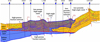 |
Fig. 14 Bottom water pressure energy invasion distribution of XC gas reservoir. |
4 Conclusion
This work intends to show a comprehensive analysis of pressure response in the vertical commingled well considering the influences of the mixed boundary in the vertical direction. Aiming at three types of the mixed boundary, we detailed analyze them by the shape of pressure response type curves and the feature value of pressure and pressure derivative. According to the analysis and application results of the vertical mixed boundary model, the following observations are highlighted:
-
The pressure response of three types mixed boundary model shows that the type of mixed boundary can be quickly captured by the shape of the pressure response curve in the log–log coordinate system and the permeability ratio of one-layer can be easily obtained by the feature value of pressure or pressure derivative.
-
The application of the mixed boundary model in the XC gas field can solve the problem of difficulty in fitting the well test curve. The combination results of geological features and interpretation parameters reveal that the existence of network fractures such as faults and high-angle fractures will cause the invasion of gas and water at the bottom-layer to form a certain degree of favorable displacement energy.
-
The interpretation results of three type wells in the XC gas field show that the composite reservoir and dual-pore reservoir characteristics on the pressure response of well test may be caused by the mixed boundary. Therefore, when the pressure response appears the features of the radial composite reservoir with poor permeability outer zone or dual-pore reservoir, the well test analysis model should be carefully selected in combination with the actual reservoir geological information.
Conflicts of interest
We declare that all co-authors participate in this manuscript. The author’s contributions are as follows: Wenyang Shi established the model and wrote the manuscript. Yuedong Yao & Mi Wang revised and improved the manuscript. Shiqing Cheng supervised this research and provided funding support. He Li & Nan Cui developed the type curves and diagnostic window figures. Chengwei Zhang organized and analyzed logging data and results. Hong Li & Kun Tu conducted field case analysis. Zhiliang Shi provided the well testing data and Saphir analysis software.
Acknowledgments
The authors thank the financial supports from the National Natural Science Foundation of China (No. 11872073) and Dr. Zhiliang Shi for providing the field data for our studies. The first author (CSC NO. 201906440196) would like to thank the China Scholarship Council for supporting his research at the School of Chemical and Process Engineering, University of Leeds, Leeds, UK. The Method and theory of this work were presented at the Journal of Petroleum Science and Engineering, Volume 194, November 2020, 107481, and the feedbacks obtained from reviews in this Journal are greatly appreciated.
References
- Shi W., Yao Y., Cheng S., Shi Z. (2020) Pressure transient analysis of acid fracturing stimulated well in multilayered fractured carbonate reservoirs: A field case in Western Sichuan Basin, China, J. Pet. Sci. Eng. 184, 1, 106462. https://doi.org/10.1016/j.petrol.2019.106462. [Google Scholar]
- Wang Y., Cheng S., Zhang K., An X. (2020) Investigation on the pressure behavior of injectors influenced by waterflood-induced fractures: field cases in Huaqing reservoir, Changqing Oilfield, China, Oil Gas Sci. Technol. - Rev. IFP Energies nouvelles 75, 20. https://doi.org/10.2516/ogst/2020013. [CrossRef] [Google Scholar]
- He Y., Qin J., Cheng S., Chen J. (2020) Estimation of fracture production and water breakthrough locations of multi-stage fractured horizontal wells combining pressure-transient analysis and electrical resistance tomography, J. Pet. Sci. Eng. 194, 11, 107479. https://doi.org/10.1016/j.petrol.2020.107479. [Google Scholar]
- Qin J., Cheng S., Li P., He Y., Lu X., Yu H. (2019) Interference well-test model for vertical well with double-segment fracture in a multi-well system, J. Pet. Sci. Eng. 183, 12, 106412. https://doi.org/10.1016/j.petrol.2019.106412. [Google Scholar]
- Luo L., Cheng S., Lee J. (2020) Characterization of refracture orientation in poorly propped fractured wells by pressure transient analysis: Model, pitfall, and application, J. Nat. Gas Sci. Eng. 79, 7, 103332. https://doi.org/10.1016/j.jngse.2020.103332. [Google Scholar]
- Lefkovits H.C., Hazebroek P., Allen E.E., Matthews C.S. (1961) A study of the behavior of bounded reservoirs composed of stratified layers, SPE J. 1, 1, 43–58. SPE-1329-G. https://doi.org/10.2118/1329-G. [Google Scholar]
- Kamal M.M., Abbaszadeh M. (2008) Transient well testing (Monograph Series), Society of Petroleum Engineers, Monograph Series Vol. 23. https://store.spe.org/Transient-Well-Testing-P380.aspx. [Google Scholar]
- Chao G., Jones J.R., Raghavan R., Lee W.J. (1994) Responses of commingled systems with mixed inner and outer boundary conditions using derivatives, SPE Form. Evalu. 9, 4, 264–271. SPE-22681-PA. https://doi.org/10.2118/22681-PA. [CrossRef] [Google Scholar]
- Shi W., Cheng S., Meng L., Gao M., Zhang J., Shi Z., Wang F., Duan L. (2020) Pressure transient behavior of layered commingled reservoir with vertical inhomogeneous closed boundary, J. Pet. Sci. Eng. 189, 6, 106995. https://doi.org/10.1016/j.petrol.2020.106995. [Google Scholar]
- Sun B., Shi W., Zhang R., Cheng S., Zhang C., Di S., Cui N. (2020) Transient behavior of vertical commingled well in vertical non-uniform boundary radii reservoir, Energies 13, 9, 2305. https://doi.org/10.3390/en13092305. [Google Scholar]
- Shi W., Yao Y., Cheng S., Shi Z., Wang Y., Zhang J., Zhang C., Gao M. (2020) Pressure transient behavior and flow regimes characteristics of vertical commingled well with vertical combined boundary: A field case in XC gas field of northwest Sichuan Basin, China, J. Pet. Sci. Eng. 194, 11, 107481. https://doi.org/10.1016/j.petrol.2020.107481. [Google Scholar]
- Yin Z., MacBeth C. (2014) Simulation model updating with multiple 4D seismic in a fault-compartmentalized Norwegian Sea Field, in: Conference Proceedings, 76th EAGE Conference and Exhibition, 11, 6, pp. 1–5. https://doi.org/10.3997/2214-4609.20141146. [Google Scholar]
- Yin Z., Ayzenberg M., MacBeth C., Feng T., Chassagne R. (2015) Enhancement of dynamic reservoir interpretation by correlating multiple 4D seismic monitors to well behavior, Interpretation 3, 2, 35–52. https://library.seg.org/doi/abs/10.1190/INT-2014-0194.1. [CrossRef] [Google Scholar]
- Suleen F., Oppert S., Chambers G., Libby L., Carley S., Alonso D., Olayomi J. (2017) Application of pressure transient analysis and 4D seismic for integrated waterflood surveillance-a deepwater case study, in: Paper Presented at SPE Western Regional Meeting, 23–27 April, Bakersfield, California. SPE-185646-MS. https://doi.org/10.2118/185646-MS. [Google Scholar]
- Suleen F., Oppert S., Lari U., Jose A. (2019) Application of pressure transient analysis and 4D seismic in evaluating and quantifying compaction in a deepwater reservoir, in: Paper Presented at SPE Western Regional Meeting, 23–26 April, San Jose, California, USA. SPE-195290-MS. https://doi.org/10.2118/195290-MS. [Google Scholar]
- Yin Z., MacBeth C., Chassagne R., Vazquez O. (2016) Evaluation of inter-well connectivity using well fluctuations and 4D seismic data, J. Pet. Sci. Eng. 145, 9, 533–547. https://doi.org/10.1016/j.petrol.2016.06.021. [Google Scholar]
- Sambo C., Iferobi C.C., Babasafari A.A., Rezaei S., Akanni O.A. (2020) The role of 4D time-lapse seismic technology as reservoir monitoring and surveillance tool: A comprehensive review, J. Nat. Gas Sci. Eng. 80, 8, 103312. https://doi.org/10.1016/j.jngse.2020.103312. [Google Scholar]
- Agarwal R.G. (1979) “Real Gas Pseudo-Time” – a new function for pressure buildup analysis of MHF gas wells, in: Paper Presented at SPE Annual Technical Conference and Exhibition, 23–26 September, Las Vegas, Nevada. SPE-8279-MS. https://doi.org/10.2118/8279-MS. [Google Scholar]
- Al-Hussainy R., Ramey H.J., Crawford P.B. (1966) The flow of real gases through porous media, J. Pet. Technol. 18, 5, 624–636. SPE-1243-A-PA. https://doi.org/10.2118/1243-A-PA. [CrossRef] [Google Scholar]
- Wang Y., Ayala L.F. (2020) Explicit determination of reserves for variable-bottomhole-pressure conditions in gas rate-transient analysis, SPE J. 25, 1, 369–390. SPE-195691-PA. https://doi.org/10.2118/195691-PA. [CrossRef] [Google Scholar]
- Bourdet D. (1985) Pressure behavior of layered reservoirs with crossflow, in: Paper Present at SPE California Regional Meeting, 27–29 March, Bakersfield, California. SPE-13628-MS. https://doi.org/10.2118/13628-MS. [Google Scholar]
- Colin MacLaurin A.M. (1748. A treatise of algebra. https://books.google.co.uk/books?id=BIrWrEEin5YC&hl=zh-CN&source=gbs_navlinks_s. [Google Scholar]
- Van Everdingen A.F., Hurst W. (1949) The application of the Laplace transformation to flow problems in reservoirs, J. Pet. Technol. 1, 12, 305–324. SPE-949305-G. https://doi.org/10.2118/949305-G. [CrossRef] [Google Scholar]
- Stehfest H. (1970) Algorithm 368: Numerical inversion of Laplace transforms [D5], Commun. ACM 13, 1, 47–49. https://dl.acm.org/doi/10.1145/361953.361969. [Google Scholar]
- Bourdet D. (2002) Chapter 2 – the analysis methods, in: Part volume of Well Ttest analysis: The use of advanced interpretation models, Handbook of Petroleum Exploration and Production 3, pp. 25–46. https://doi.org/10.1016/S1567-8032(03)80028-9. [CrossRef] [Google Scholar]
All Tables
All Figures
|
Fig. 1 (a) Tectonic map of XC gas field. (b) Reservoir profile of XC gas field. |
| In the text | |
|
Fig. 2 Physical model of two-layer mixed boundary reservoir. (a) Reservoir model. (b) Radial flow model. (c) Vertical flow model. |
| In the text | |
|
Fig. 3 Pressure response of infinite mixed boundary reservoir (two layers, one layer bounded and other infinite). (C D = 10, S = 3, κ[Ω] = κ[Θ] = 0.5, ω[Ω] = ω[Θ] = 0.5, r eD [Ω] = r eD [Θ] = 5000). |
| In the text | |
|
Fig. 4 Pressure response of equidistant mixed boundary reservoir (two layers, one layer closed and other const-pressure). (C D = 10, S = 3, κ[Ω] ≠ κ[Θ], ω[Ω] = ω[Θ] = 0.5, r eD [Ω] = r eD [Θ] = 5000). |
| In the text | |
|
Fig. 5 Pressure response of non-equidistant mixed boundary reservoir (closed boundary is near, and const-pressure boundary is far). (C D = 10, S = 3, κ[Θ] = {0.1, 0.9}, κ[Ω] = {0.1, 0.9}, ω[Ω] = ω[Θ] = 0.5, r eD [Θ] = 5000, r eD [Ω] = 500 000). |
| In the text | |
|
Fig. 6 Pressure response of non-equidistant mixed boundary reservoir (const-pressure boundary is near, and closed boundary is far). (C D = 10, S = 3, κ[Θ] = {0.1, 0.9}, κ[Ω] = {0.1, 0.9}, ω[Ω] = ω[Θ] = 0.5, r eD [Ω] = 5000, r eD [Θ] = 500 000). |
| In the text | |
|
Fig. 7 Stratified workflow base on the logging data and geological information. |
| In the text | |
|
Fig. 8 Basis and results of the stratified workflow of X10. (a) Porosity distribution of X10. (b) Permeability distribution of X10. (c) Thickness distribution of X10. (d) Pressure conductivity ratio distribution of X10. (e) Sedimentary structure map of X10. (f) Lithology profile of X10. (g) Reservoir stratification result of X10. |
| In the text | |
|
Fig. 9 Well test data of X10 and fitting curves of model r eD [Θ] & r eD [∞]. |
| In the text | |
|
Fig. 10 Basis and results of the stratified workflow of X3. (a) Porosity distribution. (b) Permeability distribution. (c) Thickness distribution. (d) Pressure conductivity ratio distribution. (e) Sedimentary structure map of X3. (f) Imaging logging of X3. (g) Lithology profile of adjacent wells X301. (h) Reservoir stratification result of X301. |
| In the text | |
|
Fig. 11 Well test data of X3 and fitting curves of model r eD [Ω] & r eD [∞]. |
| In the text | |
|
Fig. 12 Basis and results of the stratified workflow of X5. (a) Porosity distribution of X5. (b) Permeability distribution of X5. (c) Thickness distribution of X5. (d) Pressure conductivity ratio distribution of X5. (e) Sedimentary facies map of X5. (f) Imaging logging of X5. (g) Lithology profile of X5. (h) Reservoir stratification result of X5. |
| In the text | |
|
Fig. 13 Well test data of X5 and fitting curves of model r eD [Ω] & r eD [Θ]. |
| In the text | |
|
Fig. 14 Bottom water pressure energy invasion distribution of XC gas reservoir. |
| In the text | |