Regular Article
Numerical investigation on the effect of boundary conditions on the scaling of spontaneous imbibition
Department of Petroleum Engineering, Texas A&M University at Qatar, Education City, PO Box 23874, Doha, Qatar
* Corresponding author: This email address is being protected from spambots. You need JavaScript enabled to view it.
Received:
17
February
2018
Accepted:
7
September
2018
Abstract
We present a numerical validation of the scaling group presented by Schmid and Geiger ((2012) Water Resour. Res. 48, 3) for Spontaneous Imbibition (SI) through simulating a core sample bounded by the wetting fluid. We combine the results of the simulations with the semi-analytical model for counter-current spontaneous imbibition presented by Schmid et al. ((2011) Water Resour. Res. 47, 2) to validate the upscaling of laboratory experiments to field dimensions using dimensionless time. We then present a detailed parametric study on the effect of Boundary Conditions (BC) and characteristic length to compare imbibition assisted oil recovery with several types of boundary conditions. We demonstrate that oil recovery was the fastest and most efficient when all faces are open to flow. We also demonstrate that all cases scale with the non-dimensionless time suggested by Schmid and Geiger ((2012) Water Resour. Res. 48, 3) and show a close match to the numerical simulation and the semi-analytical solution. Moreover, we discuss how the effect of constructing a model with varying grid sizes and dimensions affects the accuracy of the results through comparing the results of the 2-D and 3-D models. We observe that the 3-D model proved superior in the accuracy of the results to simulate simple counter-current SI. However, we deduce that 2-D models yield satisfying enough results in a timely manner in the One End Open (OEO) and Two Ends Open (TEO) cases, compared to 3-D models which are time-consuming. We finally conclude that the non-dimensionless time of Schmid and Geiger ((2012) Water Resour. Res. 48, 3) works well with counter-current SI cases regardless of the boundary condition imposed on the core.
© A.S. Abd & N. Alyafei published by IFP Energies nouvelles, 2018
 This is an Open Access article distributed under the terms of the Creative Commons Attribution License (http://creativecommons.org/licenses/by/4.0), which permits unrestricted use, distribution, and reproduction in any medium, provided the original work is properly cited.
Nomenclature
tD : dimensionless time
k : permeability [mD]
ϕ : matrix porosity
L : core length [cm]
VB : bulk volume of the matrix block [cm3]
Ai : surface area open to imbibition in the ith direction [cm2]
 :
distance from the open surface to the center of the matrix block [cm]
:
distance from the open surface to the center of the matrix block [cm]
Qw : cumulative water imbibed [m3]
C
:
parameter that depends on the characteristics of the fluid-rock system [ ]
]
 :
derivative of the capillary dominated fractional flow function at the irreducible water saturation
:
derivative of the capillary dominated fractional flow function at the irreducible water saturation
D : capillary dispersion coefficient
F : capillary dominated fractional
kro max : maximum relative permeability of oil
krw max : maximum relative permeability of water
n : exponent for relative permeability of water curve shape
m : exponent for relative permeability of oil curve shape
Sw : water saturation
Swi : initial water saturation
Sor : residual oil saturation
krw : water relative permeability
kro : oil relative permeability
Pc : capillary pressure [Pa]
Pc entry : capillary pressure at the entrance of the pore throat [Pa]
Fs : shape factor
Lc : characteristic length [cm]
lAi : distance traveled by the imbibition front from the open surface to the no-flow boundary[cm]
t : time [s]
t* : early imbibition time [s]
tD * : dimensionless time at early imbibition time [s]
l : exponent for capillary pressure curve
1 Introduction
The physical phenomenon of imbibition is important in the understanding of fluid flow in water drive reservoirs as it directly affects water movement and areal sweep efficiency (Meng et al., 2016). Imbibition is scientifically defined as the absorption of a-wetting phase into a porous rock and can be divided into two main categories: forced and spontaneous (Ge et al., 2015). In our everyday life, we dry dishes using paper towels, or we write on a sheet of paper using ink. The physical transfer of the water into the paper towels or the ink onto the sheet of paper is described as spontaneous imbibition (Morrow and Mason, 2001). The fluid imbibes into the porous structure of the paper towel or the sheet of paper due to capillary forces. The process of spontaneous imbibition is driven by the difference in the capillary force as the spontaneous imbibition recovery is all the higher as the hydrophilicity of the rock surface is stronger (Mao et al., 2015). Different rock and fluid properties such as permeability, wettability and interfacial tension between the wetting and the non-wetting phase determine how fast the non-wetting phase would move out of the rock to be replaced by the wetting phase (Anderson, 1986). The forms of spontaneous imbibition are divided into two categories: co-current and counter-current, in which the fluid phases flow in identical and opposite directions respectively (Al-Lawati and Saleh, 1996; Bourbiaux and Kalaydjian, 1990; Iffly et al., 1972; Parsons and Chaney, 1966).
Extensive research has been concluded in the past to understand the phenomenon of spontaneous imbibition in water-wet rocks and to scale experimental data of oil recovery against dimensionless time (Bourbiaux and Kalaydjian, 1990; Cil et al., 1998; Cuiec et al., 1994; Du Prey, 1978; Hamon and Vidal 1986; Iffly et al., 1972; Rangel-German and Kovscek, 2002; Zhang et al., 1996). Upscaling imbibition assisted oil recovery as a function of dimensionless time has been of great importance to the researchers which has been exhibited through extensive experimental work that led to the development of various scaling groups. (Standnes, 2010). Moreover, scaling groups can greatly facilitate the process of predicting oil recovery from reservoirs. In other words, lab tests done on rock samples can be used to estimate macro-level oil recovery from a reservoir when integrated into field-scale simulators by the means of scaling techniques.
Several authors have proposed various scaling groups to correlate imbibition data since 1918 (Lucas, 1918; Washburn, 1921; Mattax and Kyte, 1962; Rapoport, 1955; Reis and Cil, 1993; Zhou et al., 2002; Li and Horne, 2004, 2006). However, the work of Ma et al. (1997) based on the experiments of Kazemi et al. (1992) showed the importance of using a shape factor Fs that accounts for different boundary conditions to compensate for the geometry of the matrix elements applied to reservoirs: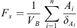 (1)where VB is the bulk volume of the matrix block,
  is the surface area open to imbibition in the ith direction,
  is the distance from the open surface to the center of the matrix block, and n is the total number of surfaces open to the imbibition.
Based on the aforementioned results, Ma et al. (1997) proposed an equation for the characteristic length to account for the variation in the profile of the fluid saturation. Kazemi et al. (1992) and Hamon and Vidal (1986) suggested the following equation: (2)where
  is the distance traveled by the imbibition front from the open surface to the no-flow boundary.
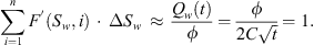
Recently, a new scaling group was derived by Schmid and Geiger (2012) based on the general exact solution of the two-phase Darcy equation for the case of counter-current imbibition (McWhorter and Sunada, 1990, 1992). This model is considered as the “master equation” for scaling spontaneous imbibition where all previously derived models appear to be special cases of this generic model:![Mathematical equation: $$ {t}_D={\left[\frac{{Q}_w(t)}{\phi {L}_c}\right]}^2={\left[\frac{2C}{\phi {L}_c}\right]}^2t $$](/articles/ogst/full_html/2018/01/ogst180052/ogst180052-eq9.gif) (3)where Qw is the cumulative water imbibed and C is a parameter that depends on the characteristics of the fluid-rock system.
(3)where Qw is the cumulative water imbibed and C is a parameter that depends on the characteristics of the fluid-rock system.
This equation is unique as all assumptions were relaxed when deriving the model except for those applicable to Darcy’s law, and it states that the total volume of the wetting phase imbibed characterizes spontaneous imbibition systems. The scaling group serves as the “master equation” for SI process, and this was proven extensively by the Schmid and Geiger (2012). The group was tested against 42 sets of different experiential data consisting of different rock properties, fluid properties and boundary conditions. The suggested group could neatly scale all the different sets into one single curve that matches the semi-analytical solution. However, the validation of the authors’ claim about the generality of their group has not been tested numerically, as extensive and detailed parametric study must be done on each rock and fluid property to confirm the scaling claim.
In their paper, Schmid and Geiger (2012) clarified that the derived solution is only valid for cases when the wetting front has not reached the end of the core or hindered any other waterfront flowing in a different direction from moving to further exposed surface areas. The time t* represents the end time in which the semi-analytical solution stops being valid because in late times the model severely fails in predicting the recovery rates. This time t* is called “early-time imbibition” and is represented by![Mathematical equation: $$ {t}^{*}={\left[\frac{L\phi }{2C{F}^\mathrm{\prime}({\mathrm{S}}_{{wir}})}\right]}^2 $$](/articles/ogst/full_html/2018/01/ogst180052/ogst180052-eq10.gif) (4)where F′(Swir) is the derivative of the capillary dominated fractional flow function at the irreducible water saturation. The derivation steps are shown in the appendix.
(4)where F′(Swir) is the derivative of the capillary dominated fractional flow function at the irreducible water saturation. The derivation steps are shown in the appendix.
Table 1 summarizes the milestones in the development of different upscaling groups, and highlights the main advantages and drawbacks of each model.
A summary of the main scaling groups devised to model spontaneous imbibition.
The primary focus of this work is to validate the latest scaling group for spontaneous imbibition developed by Schmid and Geiger (2012) through numerical modeling. The work aims to show that numerical simulation of SI processes can be done on widely available black oil simulator. The choice of such a simulator will make the process of reproducing our results easier, while providing clear guidelines on how to set up the simulation model. Most of the work done in the field of numerical SI analysis calls for the use of specialized simulation packages, or writing custom simulation codes similar to the work of Pooladi-Darvish and Firoozabadi (2000), Li and Horne (2006), and Nooruddin and Blunt (2016). However, our work generalizes the process of simulating SI to include standard commercial black oil simulators which are used widely in the reservoir simulation field. We will present various 2-D and 3-D simulation models for counter-current SI to test if imbibition recovery data scales with the non-dimensional time regardless of the boundary conditions imposed and fluid properties used. In addition, we will discuss how Schmid and Geiger (2012) is fit to scale different data sets without restriction on the boundary conditions imposed.
In this paper, we will:
-
Introduce the steps required to build the 2-D and 3-D simulation modes, and to select the optimal choice of grid size to simulate counter-current SI. This model will be used to investigate the validity of the semi-analytical solution.
-
Describe briefly the process of utilizing the semi-analytical solution to predict the oil recovery of a strongly water-wet rock and compare it with the results of the numerical simulation. The imbibition-assisted oil recovery data obtained from both the semi-analytical solution and numerical simulation will then be scaled against the dimensionless time of Schmid and Geiger (2012) to check whether it yields a good correlation independent of the rock material and/or fluid characteristics.
-
Examine carefully the imbibition time of the numerical model and confirm if the model fails in predicting the recovery for late time imbibition when recovery rates become slower at t > t*.
-
Compare the accuracy of the simulation model in 2-D and 3-D, and recommend the suitable model for each boundary condition.
2 Methodology
In this section, we will discuss the steps to build a numerical 2-D model for a water-wet core sample. This model will be used to simulate counter-current spontaneous imbibition based on the input parameters provided in Schmid et al. (2016) study and then this is compared with the semi-analytical model of Schmid et al. (2011). We will then construct the relative permeability and capillary pressure curves based on a power-law model and perform a sensitivity study with regard to the grid size of the simulation model.
2.1 Semi-analytical solution for counter-current spontaneous imbibition
We will introduce the semi-analytical solution for counter-current spontaneous imbibition developed by Schmid et al. (2011). The semi-analytical solution for spontaneous imbibition utilizes the fractional flow theory for capillary-dominated flow where displacement is controlled entirely by capillary forces. The model is initiated through a simple mass balance for two-phase flow. Using Darcy’s law, and ignoring gravitational forces and capillary back pressure, the derivation leads to the following semi-analytical solutions for counter-current imbibition as follows: (5)where D is the capillary dispersion coefficient defined as
 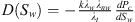 , F is the capillary dominated fractional flow function and C is an empirical constant
  . The detailed derivation for the semi-analytical solution is presented in the appendix.
In order to solve for C and F, one would have to solve the integral implicitly. However, a simple excel program utilizing the concept of backward-difference approximation through an iterative process of the unknown constant C is used (Alyafei et al., 2016; Schmid et al., 2016). This spreadsheet makes use of the following equations: (6)
(6)
 (7)
(7)
The solution process is as follows:
-
Determine F″ from a backward-differencing approximation.
-
Iteratively determine F(Sw) at a finite number n of saturation points.
-
Iterate on the constant C.
-
Keep changing C until F(Sw) converges to the correct solution.
The final value of C is obtained when equation (6) converges to 0, and equation (7) converges to 1.
2.2 Grid model and input parameters
Based on the Schmid et al. (2016) data, a strongly water-wet state case was used to serve as the basis of the numerical simulation with four different boundary conditions, which will be discussed later. The core was modeled as a rectangular prism of dimensions 7.66 cm × 2.5 cm × 2.5 cm measured in lab units. Furthermore, the model represents a conventional single porosity (20%) and single permeability (300 mD) rock sample that utilizes Cartesian gridding for property distribution.
The simulation model was developed on a commercially available black oil simulator. The number of cells used is finite in order to approximate the volume of the core. This finite number of cells will allow us to solve the flow equations in a numerical fashion. Subsequently, the most efficient number of cells in the shortest simulation time possible was determined by performing a sensitivity analysis. For this purpose, a rectangular grid was created mimicking a one-end open flow boundary in which all the sides of the core are sealed and isolated except for one end. An extra gridblock was attached to the open end of the core to serve as a water tank for the imbibition process with an equivalent volume 10 times that of the core pore volume. The water tank was set to have 100% water saturation and porosity.
Table 2 summarizes the input parameters used to calculate the semi-analytical solution for a strongly water-wet case based on Schmid et al. (2016) data.
Parameters representing a strongly water-wet Barea sandstone referenced in Schmid et al. (2016) and used to solve for the counter-current semi-analytical model.
The relative permeability curves were constructed based on the Brooks-Corey model:![Mathematical equation: $$ {k}_{{rw}}={k}_{{rw}\enspace {max}}{\left[\frac{{S}_w-{S}_{{wi}}}{1-{S}_{{wi}}-{S}_{{or}}}\right]}^n $$](/articles/ogst/full_html/2018/01/ogst180052/ogst180052-eq16.gif) (8)
(8)
![Mathematical equation: $$ {k}_{{ro}}={k}_{{ro}\enspace {max}}{\left[\frac{1-{S}_w-{S}_{{or}}}{1-{S}_{{wi}}-{S}_{{or}}}\right]}^m $$](/articles/ogst/full_html/2018/01/ogst180052/ogst180052-eq17.gif) (9)
where kro max is the maximum relative permeability of oil, krw max is the maximum relative permeability of water, n and m are the relative permeability exponents, Sw is the water saturation, Swi is the initial water saturation, Sor is the residual oil saturation, krw is water relative permeability and kro is the oil relative permeability.
(9)
where kro max is the maximum relative permeability of oil, krw max is the maximum relative permeability of water, n and m are the relative permeability exponents, Sw is the water saturation, Swi is the initial water saturation, Sor is the residual oil saturation, krw is water relative permeability and kro is the oil relative permeability.
On the other hand, the capillary pressure prediction model in a water-wet system follows the given relation:
![Mathematical equation: $$ {P}_c={P}_{{c}\enspace {entry}}{\left[\frac{{S}_w-{S}_{{wi}}}{{S}_{\mathrm{w}\enspace {@}\enspace {P}_{{c}\enspace {entry}}}-{S}_{{wi}}}\right]}^l $$](/articles/ogst/full_html/2018/01/ogst180052/ogst180052-eq19.gif) (10)where l is the capillary pressure exponent, Pc is the capillary pressure, Pc entry is the capillary pressure at the entrance of the pore throat, and
(10)where l is the capillary pressure exponent, Pc is the capillary pressure, Pc entry is the capillary pressure at the entrance of the pore throat, and  is the water saturation at the Pc entry.
The generated relative permeability and capillary pressure plots are presented in Figure 1. The semi-analytical solution obtained from equation (5) for this specific case returned a C value of 4.63 × 10⁻⁵ 
 |
Fig. 1. Capillary pressure and relative permeability for a strongly water-wet sandstone rock. The green color refers to the oil while the blue color refers to the water. The black line represents the capillary pressure curve. The data is based on the Schmid et al. (2016) study. |
2.3 Sensitivity analysis
After creating the model, the dimensions of the Cartesian grid were varied at six intervals and are shown in Table 3. The analysis of the plots of oil recovery as a function of time of both the numerical and semi-analytical solutions was the most influential factors in determining the optimal number of grids to be used in our model. It can be interpreted from Figure 2 that as the number of grids used becomes larger, the discrepancies in the oil recovery curves diminish. If we examine grid 50 × 50 × 1 and grid 100 × 100 × 1 closely, we can see that the two curves are almost overlapping compared to previous coarser grids. To quantify the difference in the results of cases 5 and 6, the Mean Squared Error (MSE) was calculated since it is the most commonly used error metric (McLean et al., 2012). It penalizes more substantial errors because squaring larger numbers has a more significant impact than squaring smaller numbers. The MSE calculation in our case returned a rather small error percentage of 0.00258%. Hence, the cutoff for the grid size is deduced to be at 50 × 50 × 1.
 |
Fig. 2. Oil recovery factors for different grid sizes. The effect of the grid size is clear from the results of the static imbibition runs. The best fit with the semi-analytical solution is achieved for a grid size of 50 × 50 × 1. |
Grid sizes investigated in the grid sensitivity analysis along with the CPU time required.
As a final validation step for the applicability of our simulation model, we plotted the semi-analytical solution corresponding to the same properties used in the simulation file. The black line representing the semi-analytical solution is observed to match the finer grid block sizes at early times where the semi-analytical solution is valid. Hence, we can say with confidence that the threshold grid size of 50 × 50 × 1 is critical where any larger grid would take much more time to simulate without any significant improvement on the accuracy of the results. This choice of grid size guarantees the convergence of the simulation results in a fashionably timed manner.
3 Results and discussion
3.1 Boundary conditions and characteristic length
Once the 50 × 50 × 1 model has been established, different boundary conditions scenarios were considered. The volume of water imbibed from the water tank into the rock sample was used to predict the recovery factors for each boundary condition studied.
The following boundary conditions were studied in the counter-current simulation case (Yildiz et al., 2006):
-
One End Open (OEO) is when most sides of the core sample are isolated, permitting the wetting phase to flow into the core through one open end located at the left side of our horizontal core (Fig. 3a).

Fig. 3. Schematic representation of the different boundary conditions considered in this study where (a) is OEO, (b) is TEO, (c) is TEC and (d) is AFO.
-
Two Ends Open (TEO) is when the top and the bottom sides in the i-direction of the core are isolated while the flow occurs throughout the whole length of the core (Fig. 3b).
-
Two Ends Closed (TEC) is when the wetting phase flows into the rock through the top and the bottom sides while isolating the entire length of the core sample (Fig. 3c).
-
All Faces Open (AFO) is when all sides of the core are exposed to the flow imbibing the wetting phase into the pores of the core sample (Fig. 3d).
During the imbibition assisted oil recovery phenomenon, the rate of oil recovered is significantly affected by the geometric elements of the matrix including the size, shape and boundary conditions applied to the core sample. Therefore, Schmid and Geiger (2012) used the characteristic length to represent different boundary conditions when scaling the SI data. Moreover, equation (2) will be used in this section to represent the different boundary conditions shown in Figure 3. Table 4 shows a summary of the formulas used to calculate the shape factor and the characteristic length for a rectangular prism (Fig. 4) representing our core for the four boundary conditions: OEO, TEC, TEO, and AFO.
 |
Fig. 4. Dimensions for a rectangular prism core sample. |
Shape factors and characteristic lengths of a rectangular prism similar to the one shown in Figure 4 with different boundary conditions (Yildiz et al., 2006).
3.2 Oil recovery for different boundary conditions
In general, the amount of recovered oil will increase as the number of faces available for imbibition increases given a specified time frame. In order to verify this statement, we plotted the recovery of oil versus time for the different boundary conditions tested: OEO, TEO, TEC, and AFO ( Fig. 5). Basing our discussion on a flow time of 15 000 s, the highest recovery, at around 52%, was achieved when all the faces of the core were exposed to water, thus enhancing the counter-current imbibition process. On the contrary, this recovery decreases to 48% when only one face is available for imbibition as in the condition of OEO. Since we are dealing with a 2-D model, both TEO and TEC have two faces open to flow and hence they are expected to have almost the same recovery factor. However, the surface area open to flow in the TEC case is along the j-direction, thus allowing the displacement of oil along the horizontal axis to be more efficient as more surface area is open to imbibition. The time needed to reach the maximum recovery in OEO is almost 15 000 s. However, the maximum recovery is reached much faster in AFO and TEC where only 200 s are needed.
 |
Fig. 5. Recovered oil for different boundary conditions produced by means of numerical simulation. The highest recovery is achieved when all faces are open to flow and thus pushing the oil out of pores effectively. |
The difference in the amount of oil recovered between the AFO and OEO boundary conditions is only 4%; however, the time required to achieve this maximum recovery varies greatly. This can be seen in Figure 6 where the time needed to fully recover the oil from the core and reach to the residual oil saturation for the OEO boundary condition is almost eight times the time taken for when the AFO condition is simulated. This confirms that the number of faces available for imbibition greatly affects the time utilized to roughly recover the same amount of oil from the different boundary conditions cases. However, the ultimate recovery will be the same in all boundary conditions if enough time is given for the water to completely displace the oil out of the core. Hence, the oil recovery for the AFO condition is the fastest to achieve when compared with all other cases.
 |
Fig. 6. Time needed to reach residual oil saturation as a function of the faces exposed to imbibition per boundary condition. It shows the maximum oil is recovered when all the faces of the core are available to exchange fluids. |
3.3 Calibration of the semi-analytical model to simulation tests
Predicting oil recovery from reservoir matrix blocks can be a tedious process. Moreover, the simulators used to calculate oil recovery from field data often face the problem of increased computing time until a satisfactory solution is converged upon. However, many researchers claim that scaling the imbibition rate through scaling laws can reduce the simulation time of the process significantly when integrated into field scale simulators (Morrow and Mason, 2001).
The counter-current imbibition results discussed earlier are hence used to evaluate the validity of a new modified so-called “master” scaling group developed by Schmid and Geiger (2012) that is independent of rock and fluid type and the wetting condition of the rock. In our study, numerical approaches were used to test the applicability of the scaling equation for the four examined boundary conditions. The semi-analytical results of the oil recovered by the spontaneous imbibition mechanism were plotted against the non-dimensional time of equation (4) on a semi-log scale. The plots presented in Figures 7a and 7b revealed the importance of normalizing the core length into different characteristic lengths per case to achieve unity in the curves. The early imbibition time t* is shown as well to indicate the region 0 < t < t* where the semi-analytical solution is valid. Table 5. shows the four boundary conditions with the characteristic length and corresponding tD equation.
 |
Fig. 7. Recovery of the oil displaced versus time. (a) Time is scaled according to the scaling group proposed by Schmid and Geiger (2012). The data did not scale up curve since the characteristic length per case was not used in the equation. (b) In this graph, we used the equation mentioned in Table 2 to calculate the characteristic length for the different cases presented in Figure 3. We can see that the data falls neatly into almost one single curve indicating that the represented length of the core should be replaced as per the boundary condition requirement. |
The volume of oil recovered was calculated based on the assumption that the volume of fluid is conserved in a counter-current spontaneous imbibition case where there is no flow across the boundaries of the system. Hence, the volume of the cumulative water imbibed into the core sample calculated from the semi-analytical solution should be equal to the volume of oil recovered from the core and is represented in the following equation from Schmid and Geiger (2012): (12)
(12)
The plots in Figure 7b indicate how the recovery curves at different boundary conditions generated using the semi-analytical solution would fall into almost one curve when the dimensionless time is used.
3.4 Testing the validity of the scaling group against the semi-analytical solution
Now, we compare the results of imbibition assisted oil recovery obtained numerically to those calculated with the semi-analytical solution. This will allow us to verify whether there will be a match in the shape of the oil recovery curves at the different boundary conditions. The plots in Figure 8 show a high agreement between the semi-analytical and the numerical solution for the different boundary conditions listed in this study. The results of the simulation scale up nicely with the dimensionless time proposed, thus validating the scaling group. Furthermore, scaling the simulation data and the average semi-analytical solution of the four cases with the dimensionless time (tD) show that both solutions fall into a neat curve. Regardless of the boundary condition imposed on the system, only a little scatter is observed around the semi-analytical solution. Notice that the solution is only valid as the condition tD < t* is satisfied.
 |
Fig. 8. Recovery of the oil displaced versus time. The numerical results are compared with the semi-analytical solution for the different boundary conditions presented in Table 2. The simulation in general shows a high agreement with the semi-analytical solution upon using the scaling group. The cases are labeled as a, b, c and d to represent OEO, TEC, TEO and AFO respectively. |
However, observing the AFO and TEC cases closely, we see that the match between the two data sets is not satisfactory and can be enhanced. One main reason for the discrepancies can be attributed to the fact that 2-D models are used for all different cases. However, in fact the TEC and AFO cases have flow coming from three different directions, and hence should be accounted for. We simulated the TEC case again while considering the dimensions of the problem, and the results were plotted in Figure 9. The results of the 3-D numerical solution showed a much better match with the semi-analytical profile as opposed to the 2-D model.
 |
Fig. 9. The plot shows the ultimate recovery of oil as function of the dimensionless time. The 3-D model shows the best fit with the semi-analytical solution but it is only valid till the early imbibition time, tD*. |
Furthermore, the AFO case was revisited. Besides simulating the process in a 3-D model, grid refining schemes were attempted to enhance the results of the 2-D model as well. Due to the fact the water in the AFO case flows into the core from 4 and 6 different directions in a 2-D and 3-D problem respectively, the 50 × 50 × 1 grid size might not be able to capture the changes in the saturation profile. For this purpose, we simulated the AFO case again with the 100 × 100 × 1 grid size model that will allow us to achieve higher accuracy in predicting recovery behavior.
The results plotted in Figure 10 show that the semi-analytical solution along with the different recovery profiles for the AFO case. We can clearly notice that the degree of correlation increased with finer grid size when the 100 × 100 × 1 model is used. Moreover, when considering a 3-D flow into the core, we get an almost perfect fit for the numerical and semi-analytical solution at early imbibition time.
 |
Fig. 10. The plot shows the ultimate recovery of oil as function of the dimensionless time. The finer grid size shows clearly a better fit with the semi-analytical solution compared to the 50 × 50 × 1 model. The fit gets even better when even finer grids are used to the areas close to the boundaries and thus allows the capturing of final saturation changes. Moreover, the 3-D model shows the best fit with the semi-analytical solution but it is only valid till the early imbibition time, tD*. |
Examining the results further, we noticed that regardless of the faces available for imbibition, the oil recovery scaled smoothly with the dimensionless groups and scattered into a narrow range of data around the average semi-analytical solution (Fig. 11). Therefore, the results of the spontaneous imbibition obtained through simulation correlate greatly with the results derived from the semi-analytical solution proposed by the new master dimensionless scaling group. The data are reduced to a single curve despite the fact that the characteristic length varies greatly from one case to the other (0.81 cm < Lc < 7.66 cm).
 |
Fig. 11. The plot shows normalized oil recovery factor and is plotted against time. Time is scaled according to Schmid and Geiger (2012) model resulting in the data to collapse into one curve on a semi-log scale. The scatter of the data is reasonable and within the range of the semi-analytical solution as can be seen in the plot. The semi-analytical solution is valid as long as the dimensionless time satisfies the condition tD < tD* presented in the introduction earlier. Although the oil flow in the AFO case is considerably faster compared to the other cases, the results still converge into almost a single curve. |
The simulation results were also plotted against different scaling groups to compare the quality of scaling between different models. In this analysis, five different scaling groups, including Schmid and Geiger (2012) group were used to calculate the dimensionless time for each of the simulated cases. The main difference between the groups is that Ma et al. (1997), Zhou et al. (2002) and Schmid and Geiger (2012) utilize the concept of the characteristic length, while Mattax and Kyte (1962) and Reis and Cil (1993) do not. The five different scaling groups were plotted on five separate plots shown in Figures 12a–e. The simulation parameters were all fixed except for the changing boundary condition which was exhibited in each case. We notice that whenever the characteristic length suggested by Ma et al. (1997) is used, the choice of scaling group does not matter given that all the parameters other than the boundary conditions are fixed. Early scaling groups such as Mattax and Kyte (1962) and Reis and Cil (1993) fail to scale the data as opposed to the lately developed scaling groups.
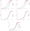 |
Fig. 12. The plots show ultimate recovered oil versus dimensionless time for different scaling groups: (a) Reis and Cil (1993); (b) Mattax and Kyte (1962); (c) Zhou et al. (2002); (d) Ma et al. (1997) and (e) Schmid and Geiger (2012). |
However, this comparison does not show that Schmid and Geiger (2012) is indeed universal in scaling SI data, as the control parameter was the boundary condition which can be scaled by a group that utilizes the concept of the characteristic length. For this purpose, we constructed 16 different simulation cases with random porosity, permeability, length, viscosity ratio, boundary conditions and rock properties. The goal is to see whether Schmid and Geiger (2012) scaling group will be able to scale the data with varying range of rock and fluid parameters into a single smooth curve. The results of the scaling will be compared with Ma et al. (1997) which is considered amongst the best scaling groups for counter-current SI. The synthesized data sets are summarized in Table 6 below.
The rock and fluid parameters used to synthesize the data sets for numerical modeling.
Upon simulating the 16 different cases, the numerical results were used to calculate the dimensionless time of the two tested groups, and the ultimate recovery curves were plotted on a semi-logarithmic scale in Figures 13a and b. The curves scaled by Ma et al. (1997) in Figure 13a show great discrepancies between the different curves and the data do not scale smoothly. The only profiles that stack on top of each others are S1, S2, S3 and S4, where only the boundary condition was varied. However, changing the porosity or the permeability values even slightly resulted in a mismatch proving the inability of Ma et al. (1997) to scale all of the data. On the other hand, we notice while observing Figure 13b the all the data sets fall into almost one curve collapsing on top of each. The huge variations in rock and fluid properties and relative permeability profile did not diminish the ability of Schmid and Geiger (2012) group in scaling the 16 samples. As we stated earlier, this scaling law is considered the master equation for fitting spontaneous imbibition data in both water-wet and mixed-wet systems. The superiority of the scaling group over the previously developed laws was proven Schmid and Geiger (2012) through testing the results of scaling the oil recovery analytically against 45 published experimental results with different wettability conditions, viscosity ratios and boundary conditions (Bourbiaux and Kalaydjian, 1990; Fischer et al., 2006; Hamon and Vidal, 1986; Hatiboglu and Babadagli, 2007; Zhou et al., 2002). The scaling group showed a high agreement with the experimental results thus proving its validity for a wide range of diverse data. The numerical analysis that we performed validates this conclusion.
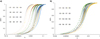 |
Fig. 13. The plots show ultimate recovered oil versus dimensionless time for different scaling groups: (a) Ma et al. (1997) does not scale the different data sets and fail to converge the result into one single curve (b) Schmid and Geiger (2012) scales the 16 different data sets into one single curve validating its universal applicability. |
3.5 Effect of grid dimensions on simulation results
In this work, a numerical investigation was performed on a 2-D grid model. However, the dimensions of the grid play a big role in the convergence of the simulator and thus affect the quality of the results; the finer the grids, the more accurate the results are but more time consuming the process is.
The base model was created using a 50 × 50 × 1 Cartesian grid. The model was varied between 1-D grid of 50 × 1 × 1 blocks and a 3-D grid of 50 × 50 × 50 blocks using the TEO boundary condition. It was noticed when running the models that the time exhausted by the simulator to run the 3-D model was around 760 s, almost five times slower than the 2-D model. The 1-D model, on the other hand, hardly took any to run with a CPU time of 5.4 s. This validates our assumption that finer grids require more time simulation time to converge. But the fundamental question is that if this finer model will produce better results when compared to the base model. Although time is of the essence in simulations, one can sacrifice extra processing time if the quality of the output is unique and accurate. For this purpose, we plotted the oil recovery versus time for the different grid sizes used (Fig. 14). The results were expected as the 1-D model showed high discrepancies when compared to the 2-D and 3-D cases. On the contrary, oil recovered using the latter model showed a close correlation between the data sets as the MSE between the 2-D and the 3-D models was around 0.0049% only. The plot shows that both curves almost overlap leading us to believe that the additional simulation time utilized to step up from a 2-D model did not affect the results. The final output of the numerical modeling is reasonably close, showing the superiority of the 2-D models in predicting the oil recovery from the water-wet rock for a counter-current spontaneous imbibition case within reasonable time limits. However, as shown earlier, only 3-D model could get a fit with the semi-analytical solution for both TEC and AFO cases. Hence, it recommended to use 2-D models to represent the OEO and TEO cases as the direction of the flow is constricted in the i and j direction, with the height bearing no influence on the fluid movement. However, more complex cases like TEC and AFO are recommended to utilize the approach of the 3-D model presented in this study.
 |
Fig. 14. The plot shows recovered oil versus time for different grid sizes. There is a significant difference in the amount of oil recovered when you move from 1-D to 2-D. However, this change is minimal between 2-D and 3-D models. This could be attributed to the fact the maximum oil recovery is already reached and thus using 2-D models in satisfactory in this TEO case. |
4 Conclusions and recommendations
The results of the numerical study presented in this work provide a useful insight into the Schmid and Geiger (2012) scaling group and its capability to correlate simulation results with the analytical solution in an efficient and easy manner compared to the early upscaling techniques. The following conclusions can be drawn from this work:
-
The scaling equation developed by Schmid and Geiger (2012) used for upscaling oil recovery data significantly reduced the complexity of the mathematical operations needed to predict the oil recovery from the analytical solution. The parameters governing spontaneous imbibition are all honored implicitly in the dimensionless time.
-
Numerical simulations were conducted on different boundary conditions for core samples, showing that the imbibition rate is affected by the characteristic length of the geometric family of the core sample. The rate of the imbibition increases with all surface areas open to fluid exchange. The time required to achieve maximum recovery was the fastest in the AFO systems.
-
The number of grids used to simulate a 2-D or 3-D flow did not affect the results of the oil recovery significantly. It is advised to use a 2-D model if the OEO and TEO boundary conditions for water-wet counter current spontaneous imbibition are studied. Other boundary conditions such as AFO and TEC will require 3-D simulation models.
-
A simple variation in the rock and fluid properties proved that scaling group is valid for a wide range of data. However, a detailed parametric study is needed to examine various parameters included in the scaling group explicitly, or in the analytical solution implicitly that might affect the quality of the scaling. The effects of viscosity, capillary pressure, endpoint relative permeability and initial water saturation all must be considered to check whether they have a direct impact on the scaling group.
Acknowledgments
We would like to thank Texas A&M University at Qatar for funding this project.
References
- Al-Lawati S., Saleh S. (1996) Oil recovery in fractured oil reservoirs by low IFT imbibition process. SPE Annual Technical Conference and Exhibition, http://dx.doi.org/10.2118/36688-ms [Google Scholar]
- Alyafei N., Al-Menhali A., Blunt M. (2016) Experimental and analytical investigation of spontaneous imbibition in water-wet carbonates, Transp. Porous Media 115, 1, 189–207. http://dx.doi.org/10.1007/s11242-016-0761-4 [Google Scholar]
- Anderson W. (1986) Wettability literature survey – Part 2: wettability measurement, J. Pet. Technol. 38, 11, 1246–1262. http://dx.doi.org/10.2118/13933-pa [Google Scholar]
- Bourbiaux B., Kalaydjian F. (1990) Experimental study of cocurrent and countercurrent flows in natural porous media, SPE Reserv. Eng. 5, 3, 361–368. http://dx.doi.org/10.2118/18283-pa [CrossRef] [Google Scholar]
- Cil M., Reis J., Miller M., Misra D. (1998) An examination of countercurrent capillary imbibition recovery from single matrix blocks and recovery predictions by analytical matrix/fracture transfer functions. SPE Annual Technical Conference and Exhibition. http://dx.doi.org/10.2118/49005-ms . [Google Scholar]
- Cuiec L., Bourbiaux B., Kalaydjian F. (1994) Oil recovery by imbibition in low-permeability chalk, SPE Form. Eval. 9, 3, 200–208. http://dx.doi.org/10.2118/20259-pa [CrossRef] [Google Scholar]
- Du Prey E. (1978) Gravity and capillarity effects on imbibition in porous media, SPE J 18, 3, 195–206. http://dx.doi.org/10.2118/6192-pa [Google Scholar]
- Fischer H., Wo S., Morrow N. (2006) Modeling the Effect of Viscosity Ratio on Spontaneous Imbibition, SPE Reservoir Evaluation & Engineering 11, 3, 577–589. http://dx.doi.org/10.2118/102641-pa [CrossRef] [Google Scholar]
- Ge H., Yang L., Shen Y., Ren K., Meng F., Ji W., Wu S. (2015) Experimental investigation of shale imbibition capacity and the factors influencing loss of hydraulic fracturing fluids, Petrol. Sci. 12, 4, 636–650. http://dx.doi.org/10.1007/s12182-015-0049-2 [CrossRef] [Google Scholar]
- Hamon G., Vidal J. (1986) Scaling-up the capillary imbibition process from laboratory experiments on homogeneous and heterogeneous samples. European Petroleum Conference. http://dx.doi.org/10.2118/15852-ms [Google Scholar]
- Hatiboglu C., Babadagli T. (2007) Oil recovery by counter-current spontaneous imbibition: Effects of matrix shape factor, gravity, IFT, oil viscosity, wettability, and rock type, J. Petrol. Sci. Eng. 59, 1-2, 106–122. http://dx.doi.org/10.1016/j.petrol.2007.03.005 [CrossRef] [Google Scholar]
- Iffly R., Rousselet D., Vermeulen J. (1972) Fundamental study of imbibition in fissured oil fields. Fall Meeting of the Society of Petroleum Engineers of AIME. http://dx.doi.org/10.2118/4102-ms [Google Scholar]
- Kazemi H., Gilman J., Elsharkawy A. (1992) Analytical and numerical solution of oil recovery from fractured reservoirs with empirical transfer functions (includes associated Papers 25528 and 25818), SPE Reserv. Eng. 7, 2, 219–227. http://dx.doi.org/10.2118/19849-pa [CrossRef] [Google Scholar]
- Li K., Horne R. (2004) An analytical scaling method for spontaneous imbibition in gas/water/rock systems, SPE J. 9, 3, 322–329. http://dx.doi.org/10.2118/88996-pa [CrossRef] [Google Scholar]
- Li K., Horne R. (2006) Generalized scaling approach for spontaneous imbibition: An analytical model, SPE Reserv. Evalu. Eng. 9, 3, 251–258. http://dx.doi.org/10.2118/77544-pa [CrossRef] [Google Scholar]
- Lucas R. (1918) Ueber das Zeitgesetz des kapillaren Aufstiegs von Flüssigkeiten, Kolloid-Zeitschrift 23, 1, 15–22. http://dx.doi.org/10.1007/bf01461107 [CrossRef] [Google Scholar]
- Mao H., Qiu Z., Shen Z., Huang W. (2015) Hydrophobic associated polymer based silica nanoparticles composite with core-shell structure as a filtrate reducer for drilling fluid at utra-high temperature, Journal Of Petroleum Science And Engineering 129, 1–14. http://dx.doi.org/10.1016/j.petrol.2015.03.003 [CrossRef] [Google Scholar]
- Ma S., Morrow N. R., Zhang X. (1997) Generalized scaling of spontaneous imbibition data for strongly water-wet systems, J. Petrol. Sci. Eng. 18, 3-4, 165–178. [Google Scholar]
- Mattax C., Kyte J. (1962) Imbibition oil recovery from fractured, water-drive reservoir, SPE J. 2, 2, 177–184. http://dx.doi.org/10.2118/187-pa [Google Scholar]
- McLean K., Wu S., McAuley K. (2012) Mean-squared-error methods for selecting optimal parameter subsets for estimation, Ind. Eng. Chem. Res. 51, 17, 6105–6115. http://dx.doi.org/10.1021/ie202352f [Google Scholar]
- McWhorter D., Sunada D. (1990) Exact integral solutions for two-phase flow, Water Resour. Res. 26, 3, 399–413. http://dx.doi.org/10.1029/wr026i003p00399 [Google Scholar]
- McWhorter D., Sunada D. (1992) Reply [to “Comment on ‘Exact integral solutions for two-phase flow’ by David B. McWhorter and Daniel K. Sunada”], Water Resour. Res. 28, 5, 1479–1479. http://dx.doi.org/10.1029/92wr00474 [Google Scholar]
- Meng Q., Liu H., Wang J., Zhang H. (2016) Effect of wetting-phase viscosity on cocurrent spontaneous imbibition. Energy Fuels 30, 835–843, http://dx.doi.org/10.1021/acs.energyfuels.5b02321 [Google Scholar]
- Morrow N., Mason G. (2001) Recovery of oil by spontaneous imbibition, Curr. Opin. Colloid Interface Sci. 6, 4, 321–337. http://dx.doi.org/10.1016/s1359-0294(01)00100-5 [Google Scholar]
- Nooruddin H., Blunt M. (2016) Analytical and numerical investigations of spontaneous imbibition in porous media, Water Resour. Res. 52, 9, 7284–7310. http://dx.doi.org/10.1002/2015wr018451 [Google Scholar]
- Parsons R., Chaney P. (1966) Imbibition model studies on water-wet carbonate rocks, SPE J. 6, 1, 26–34. http://dx.doi.org/10.2118/1091-pa [Google Scholar]
- Pooladi-Darvish M., Firoozabadi A. (2000) Cocurrent and Countercurrent Imbibition in a Water-Wet Matrix Block, SPE J. 5, 1, 3–11. http://dx.doi.org/10.2118/38443-pa [CrossRef] [Google Scholar]
- Rangel-German E., Kovscek A. (2002) Experimental and analytical study of multidimensional imbibition in fractured porous media, J. Petrol. Sci. Eng. 36, 1–2, 45–60. http://dx.doi.org/10.1016/s0920-4105(02)00250-4 [CrossRef] [Google Scholar]
- Rapoport L.A. (1955) Scaling laws for use in design and operation of water-oil flow models, Trans. AIME 204, 143–150. [Google Scholar]
- Reis J., Cil M. (1993) A model for oil expulsion by counter-current water imbibition in rocks: One-dimensional geometry, J. Petrol. Sci. Eng. 10, 2, 97–107. http://dx.doi.org/10.1016/0920-4105(93)90034-c [CrossRef] [Google Scholar]
- Schmid K., Geiger S. (2012) Universal scaling of spontaneous imbibition for water-wet systems, Water Resour. Res. 48, 3, W03507 . http://dx.doi.org/10.1029/2011wr011566 [Google Scholar]
- Schmid K., Geiger S., Sorbie K. (2011) Semianalytical solutions for cocurrent and countercurrent imbibition and dispersion of solutes in immiscible two-phase flow, Water Resour. Res. 47, 2. http://dx.doi.org/10.1029/2010wr009686 [CrossRef] [PubMed] [Google Scholar]
- Schmid K., Alyafei N., Geiger S., Blunt M. (2016) Analytical solutions for spontaneous imbibition: Fractional-flow theory and experimental analysis, SPE J. 21, 6, 2308–2316. http://dx.doi.org/10.2118/184393-pa [CrossRef] [Google Scholar]
- Standnes D. (2010) Scaling group for spontaneous imbibition including gravity, Energy Fuels 24, 5, 2980–2984. http://dx.doi.org/10.1021/ef901563p [Google Scholar]
- Washburn E. (1921) The dynamics of capillary flow, Phys. Rev. 17, 3, 273–283. http://dx.doi.org/10.1103/physrev.17.273 [Google Scholar]
- Yildiz H., Gokmen M., Cesur Y. (2006) Effect of shape factor, characteristic length, and boundary conditions on spontaneous imbibition, J. Petrol. Sci. Eng. 53, 3–4, 158–170. http://dx.doi.org/10.1016/j.petrol.2006.06.002 [CrossRef] [Google Scholar]
- Zhang X., Morrow N., Ma S. (1996) Experimental verification of a modified scaling group for spontaneous imbibition, SPE Reserv. Eng. 11, 4, 280–285. http://dx.doi.org/10.2118/30762-pa [CrossRef] [Google Scholar]
- Zhou D., Jia L., Kamath J., Kovscek A. (2002) Scaling of counter-current imbibition processes in low-permeability porous media, J. Petrol. Sci. Eng. 33, 1–3, 61–74. http://dx.doi.org/10.1016/s0920-4105(01)00176-0 [CrossRef] [Google Scholar]
Appendix
The derivation of the semi-analytical solution of spontaneous and the scaling group is described in details in the work of Schmid et al. (2011) and Schmid and Geiger (2012). We will present a summarized overview of the mains steps in the model development.
We start from the wetting phase conversation equation assuming a 1-D flow of two immiscible and incompressible fluids: (A.1)
(A.1)
From the multiphase Darcy’s law, we write two equations representing the velocity of the wetting and the non-wetting phases respectively: (A.2)
(A.2)
 (A.3)
(A.3)
Since  and
and  , and ignoring the gravitational forces, we rewrite
  for counter-current imbibition as:
![Mathematical equation: $$ {q}_w=\frac{k{\lambda }_w{\lambda }_{{nw}}}{{\lambda }_t}\left[\frac{\partial {P}_c}{{\partial x}}\right]. $$](/articles/ogst/full_html/2018/01/ogst180052/ogst180052-eq29.gif) (A.4)
(A.4)
Note that for counter-current flow, qw = −qnw.
Now, if substitute the velocity equations back into equation (A.1), we get:![Mathematical equation: $$ \phi \frac{\partial {S}_w}{{\partial t}}=\frac{\partial }{{\partial x}}\left[D\left({S}_w\right)\frac{\partial {S}_w}{{\partial x}}\right] $$](/articles/ogst/full_html/2018/01/ogst180052/ogst180052-eq30.gif) (A.5)where the capillary dispersion term is:
(A.5)where the capillary dispersion term is: (A.6)
(A.6)
An analogy to Buckley-Leverett function is used to propose that a solution  scales with square root of time:
  (A.7)
(A.7)
Using this definition in equation (A.7), we rewrite equation (A.5) to become: ![Mathematical equation: $$ \omega \frac{\partial {S}_w}{{\partial \omega }}+2\frac{\partial }{{\partial \omega }}\left[D\left({S}_w\right)\frac{\partial {S}_w}{{\partial \omega }}\right]=0. $$](/articles/ogst/full_html/2018/01/ogst180052/ogst180052-eq34.gif) (A.8)
(A.8)
Also, from the Buckley-Leverett analogy we state that for some capillary fractional flow F (1 ≥ F ≥ 0) and constant C definer earlier: (A.9)
(A.9)
Hence, if we take the derivate of equation (A.9) with respect to water saturation, we get: (A.10)
Substituting equations (9) and (10) to equation (8), and defining  and
and  , we obtain:
 (A.11)
Formally, this is a semi-analytical solution to the equations, since they define F and hence the whole solution.
The scaling group is based on the frontal movement of the wetting phase: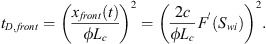 (A.12)
The dimensionless time can be further interpreted as: (A.13)
Hence, the dimensionless time becomes: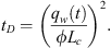 (A.14)
All Tables
Parameters representing a strongly water-wet Barea sandstone referenced in Schmid et al. (2016) and used to solve for the counter-current semi-analytical model.
Grid sizes investigated in the grid sensitivity analysis along with the CPU time required.
Shape factors and characteristic lengths of a rectangular prism similar to the one shown in Figure 4 with different boundary conditions (Yildiz et al., 2006).
The rock and fluid parameters used to synthesize the data sets for numerical modeling.
All Figures
|
Fig. 1. Capillary pressure and relative permeability for a strongly water-wet sandstone rock. The green color refers to the oil while the blue color refers to the water. The black line represents the capillary pressure curve. The data is based on the Schmid et al. (2016) study. |
| In the text | |
|
Fig. 2. Oil recovery factors for different grid sizes. The effect of the grid size is clear from the results of the static imbibition runs. The best fit with the semi-analytical solution is achieved for a grid size of 50 × 50 × 1. |
| In the text | |
|
Fig. 3. Schematic representation of the different boundary conditions considered in this study where (a) is OEO, (b) is TEO, (c) is TEC and (d) is AFO. |
| In the text | |
|
Fig. 4. Dimensions for a rectangular prism core sample. |
| In the text | |
|
Fig. 5. Recovered oil for different boundary conditions produced by means of numerical simulation. The highest recovery is achieved when all faces are open to flow and thus pushing the oil out of pores effectively. |
| In the text | |
|
Fig. 6. Time needed to reach residual oil saturation as a function of the faces exposed to imbibition per boundary condition. It shows the maximum oil is recovered when all the faces of the core are available to exchange fluids. |
| In the text | |
|
Fig. 7. Recovery of the oil displaced versus time. (a) Time is scaled according to the scaling group proposed by Schmid and Geiger (2012). The data did not scale up curve since the characteristic length per case was not used in the equation. (b) In this graph, we used the equation mentioned in Table 2 to calculate the characteristic length for the different cases presented in Figure 3. We can see that the data falls neatly into almost one single curve indicating that the represented length of the core should be replaced as per the boundary condition requirement. |
| In the text | |
|
Fig. 8. Recovery of the oil displaced versus time. The numerical results are compared with the semi-analytical solution for the different boundary conditions presented in Table 2. The simulation in general shows a high agreement with the semi-analytical solution upon using the scaling group. The cases are labeled as a, b, c and d to represent OEO, TEC, TEO and AFO respectively. |
| In the text | |
|
Fig. 9. The plot shows the ultimate recovery of oil as function of the dimensionless time. The 3-D model shows the best fit with the semi-analytical solution but it is only valid till the early imbibition time, tD*. |
| In the text | |
|
Fig. 10. The plot shows the ultimate recovery of oil as function of the dimensionless time. The finer grid size shows clearly a better fit with the semi-analytical solution compared to the 50 × 50 × 1 model. The fit gets even better when even finer grids are used to the areas close to the boundaries and thus allows the capturing of final saturation changes. Moreover, the 3-D model shows the best fit with the semi-analytical solution but it is only valid till the early imbibition time, tD*. |
| In the text | |
|
Fig. 11. The plot shows normalized oil recovery factor and is plotted against time. Time is scaled according to Schmid and Geiger (2012) model resulting in the data to collapse into one curve on a semi-log scale. The scatter of the data is reasonable and within the range of the semi-analytical solution as can be seen in the plot. The semi-analytical solution is valid as long as the dimensionless time satisfies the condition tD < tD* presented in the introduction earlier. Although the oil flow in the AFO case is considerably faster compared to the other cases, the results still converge into almost a single curve. |
| In the text | |
|
Fig. 12. The plots show ultimate recovered oil versus dimensionless time for different scaling groups: (a) Reis and Cil (1993); (b) Mattax and Kyte (1962); (c) Zhou et al. (2002); (d) Ma et al. (1997) and (e) Schmid and Geiger (2012). |
| In the text | |
|
Fig. 13. The plots show ultimate recovered oil versus dimensionless time for different scaling groups: (a) Ma et al. (1997) does not scale the different data sets and fail to converge the result into one single curve (b) Schmid and Geiger (2012) scales the 16 different data sets into one single curve validating its universal applicability. |
| In the text | |
|
Fig. 14. The plot shows recovered oil versus time for different grid sizes. There is a significant difference in the amount of oil recovered when you move from 1-D to 2-D. However, this change is minimal between 2-D and 3-D models. This could be attributed to the fact the maximum oil recovery is already reached and thus using 2-D models in satisfactory in this TEO case. |
| In the text | |