Regular Article
Downward flow of proppant slurry through curving pipes during horizontal well fracturing
1
College of Electromechanical Engineering, Qingdao University of Science and Technology, Qingdao
266061, China
2
Geo-Energy Research Institute, Qingdao University of Science and Technology, Qingdao
266061, China
* Corresponding author: Cette adresse e-mail est protégée contre les robots spammeurs. Vous devez activer le JavaScript pour la visualiser.
Received:
24
January
2018
Accepted:
5
July
2018
Abstract
The transport of proppant-fracturing fluid mixture in a fracturing pipe can significantly affect the final proppant placement in a hydraulic fracture in horizontal well fracturing. To improve the understanding of the hydrodynamic performance of proppants in a curving fracturing pipe, a modified two-layer transport model was proposed by taking the viscoelastic properties of carrier fluid into consideration. Fluid temperature was determined by an energy equation in order to accurately characterize its rheological properties, and the Chang–Darby model was used to represent the viscosity-shear rate relationship. The flow pattern of particle-fluid mixture in a curving fracturing pipe was investigated, the effects of particle and fluid properties and injection parameters were analyzed, and a flow pattern map was established. Three transport stages are observed: (1) particles keep suspended in the carrier fluid at small inclined angle; (2) a small number of particles settle and accumulate on pipe bottom to form a particle bed load flow at intermediate inclined angle; (3) numerous particles settle out of carrier fluid and the particle bed quickly develops in an approximate horizontal pipe. The transition processes between different stages were observed, and the transition velocity from particle bed load flow to full suspension flow increases with the increase in inclined angle. However, an inverse transition phenomenon occurs at intermediate inclined angle, where the full suspension flow inversely turns into particle bed load flow with the increase in injected velocity.
© G. Zhang and K. Chao, published by IFP Energies nouvelles, 2018
 This is an Open Access article distributed under the terms of the Creative Commons Attribution License (http://creativecommons.org/licenses/by/4.0), which permits unrestricted use, distribution, and reproduction in any medium, provided the original work is properly cited.
Nomenclature
SymbolsA : Pipe cross-sectional area (m2)
A h : Cross-sectional area of suspension layer (m2)
A b : Cross-sectional area of particle bed (m2)
C 0 : Injected concentration of particle-fluid mixture
C(y): Particle volumetric concentration in the position (y)
C D : Drag coefficient
C h : Mean particle volumetric concentration of suspension layer
C b : Particle volumetric concentration of particle bed
C pl : Specific heat at constant pressure for slick-water (J/kg·°C)
C ps : Specific heat at constant pressure for particle (J/kg·°C)
d p : Particle diameter (m)
D : Pipe inner diameter (m)
 :
Pressure gradient (Pa/m)
:
Pressure gradient (Pa/m)
f : Dry friction coefficient between particle bed and pipe wall
f m : Friction coefficient between suspension layer and pipe wall or particle bed
f p : Friction coefficient for polymer solutions
f s : Friction coefficient for solvent
F b : Friction force between particle bed and pipe wall (N)
F bd : Dry friction force between particle bed and pipe wall (N)
F bl : Hydrodynamic retardation force between particle bed and pipe wall (N)
g : Gravitational acceleration (m/s2)
K : Consistency coefficient (Pa s n )
L : Radius of curvature of a curving pipe (m)
m : Chang–Darby rheological model parameter
n : Flow behavior index
N De : Deborah number
N Res : Reynolds number
R : Radius of curvature for curving segment (m)
R t : Pipe heat resistance ([W/(m·°C)]−1)
S h : Contact perimeter between suspension layer and pipe wall (m)
S hb : Contact perimeter between suspension layer and particle bed (m)
T : Mixture temperature (°C)
T 0 : Injected temperature (°C)
T e : Environment temperature (°C)
U 0 : Injected velocity of particle-fluid mixture (m/s)
U h : Mean flow rate of suspension layer (m/s)
U b : Flow rate of moving particle bed (m/s)
V s : Particle terminal settling velocity (m/s)
VF: Settling velocity factor
y : The position in the pipe at the vertical coordinate (m)
y b : Particle bed height (m)
Greek symbols
Δ: Pipe roughness (mm)
Δ/D : Relative pipe roughness
α : Inclined angle of a curving pipe (°)
ε : Diffusion coefficient
ζ : Characteristic time constant of the fluid in Darby–Chang model (s)
θ b : Angle of particle bed (°)
λ : Relaxation time of polymer solutions (s)
μ 0 : Zero shear rate viscosity (Pa s)
μ ∞ : Infinite shear rate viscosity (Pa s)
μ a : Apparent viscosity (Pa s)
μ s : Solvent viscosity (Pa s)
ρ b : Density of particle bed (kg/m3)
ρ h : Density of suspension layer (kg/m3)
ρ l : Carrier fluid density (kg/m3)
ρ m : Suspension layer density (kg/m3)
ρ p : Polymer solution density (kg/m3)
ρ s : Particle density (kg/m3)
τ h : Shear stress between suspension layer and pipe wall (N/m)
τ hb : Shear stress between suspension layer and particle bed (N/m)
φ : Inner friction angle (°)
1 Introduction
In petroleum industry, the unconventional resources, such as shale gas and tight oil, have been widely developed world wide, which changes to be the focus of considerable attention as primary energy sources (Zou et al., 2015). However, because the permeability of unconventional reservoirs is extremely low, hydraulic fracturing treatments are necessary to commercially develop shale gas and tight oil (Arthur et al., 2009; Sovacool, 2014). During hydraulic fracturing treatments, high pressure fracturing fluid is first injected into a well to initiate and propagate a fracture, and in order to keep open of the hydraulic fracture, proppant load fracturing fluid is subsequently injected. The injected proppant particles settle out of the carrier fracturing fluid and accumulate on the bottom of a fracture to prohibit it from closing (Zhang et al., 2017). Since the production of a stimulated well depends on the conductivity of a hydraulic fracture, which is governed by the placement of proppant particles, it is of significant importance to accurately predict proppant transport performance in a hydraulic fracture.
Two key technologies of horizontal well completion and slick-water fracturing fluid play important role on developing unconventional resources (Brown et al., 2011; Palisch et al., 2010; Roussel and Sharma, 2011). For horizontal well fracturing, the proppant load fracturing fluid transports a long distance in a fracturing pipe before entering a hydraulic fracture. However, since the viscosity of slick-water is low, proppant particles quickly settle out of fracturing fluid, this can significantly change the flow pattern of particle-fluid mixture in a fracturing pipe. Therefore, the transport performance of proppant particles in a fracturing pipe affects a lot on their transport in a fracture, and the hydrodynamic behavior of proppant particles in a fracturing pipe must be accurately described. During horizontal well fracturing, the particle-fluid mixture first transports through a vertical segment and then enters a horizontal segment before entering a fracture as shown in Figure 1, and between the vertical and horizontal segments, the mixture must pass a transitional curving pipe, which connects the vertical and horizontal segments. In the vertical segment, an approximate homogeneous full suspension flow is observed. However, proppant particles may settle out of fracturing fluid and accumulate on pipe bottom to form a particle bed after departing the vertical segment. Therefore, it is of significant importance to investigate the hydrodynamic performance of proppant load slurry transport in non-vertical curving pipe, the inclined angle of which varies from 0° to 90° (horizontal segment).
 |
Fig. 1. Schematic of a hydraulic fracturing in a horizontal well. |
Although particle-fluid flow has been commonly studied in many engineering fields of chemical (Marfaing et al., 2017), agriculture, food, hydrology and petroleum, etc., due to the complicated interaction of particles-fluid and inter-particles, it is difficult to accurately represent the hydrodynamic performance of particles. Pseudo-fluid model is first established for dilute solid-fluid flow, and the mixture is assumed to be viscous incompressible fluid with the density and viscosity as a function of particle volumetric concentration (Noetinger, 1989; Pearson, 1994). However, because some particles settle out of carrier fluid and accumulate on pipe bottom, a multi-layer flow pattern is observed (Matoušek, 2009). Doron et al. (1987) observed a particle bed load flow during solid-fluid transport experiments in a horizontal pipe, a heterogeneous suspension layer is at pipe top while a particle bed forms on pipe bottom, which keeps stationary or moving. A two-layer model was proposed by Doron et al. to represent the transport process, and good agreement between measured pressure gradient and predicted values from the two-layer model is obtained. The particle bed load flow of particle-fluid mixture in horizontal or high deviated pipes has been commonly investigated, and a three-layer flow pattern (stationary particle bed, moving particle bed and suspension layer) even occurs at very low flow velocity (Doron and Barnea, 1993, 1995; Ravelet et al., 2013).
Since the injected rate of proppant load fracturing fluid is very high, no stationary particle bed can form on the bottom of a fracturing pipe, so the two-layer model is used to model the hydrodynamic transport process. In drilling engineering, the particle bed load flow model is used to model the upward flow of cuttings (Cho et al., 2002; Ramadan et al., 2005; Ribeiro et al., 2017). However, best to our knowledge, few has been done to investigate aslant downward transport of particle-fluid mixture. In this work, the two-layer transport model is modified by considering the viscoelastic properties of carrier fluid, the variation of flow pattern of particle-fluid mixture in a curving pipe against inclined angle is investigated, and a flow pattern map is established.
2 Models
2.1 Two-layer flow model
The two-layer transport model established by Doron and Barnea (Doron et al., 1987) is applied to model downward flow of particle-fluid mixture through a curving pipe. The schematic for the two-layer flow is shown in Figure 2. A particle bed forms on pipe bottom, which keeps stationary or moves along the pipe, while a particle-fluid heterogeneous suspension layer is at the top.
 |
Fig. 2. Geometric schematic of two-layer particle-fluid mixture flow. |
During hydraulic fracturing treatments, the injected rate of proppant slurry is very high, because small proppant particles cause small settling velocities compared with the flow velocity of carrier fluid, the slippage velocity between fluid and particles is ignored. Since one of important parameters to describe the transport behavior of particle-fluid mixture is the height of particle bed, a curvilinear abscissa along the pipe axis is used in this work, and the continuity equations for solid phase and fluid phase are shown in equations (1) and (3), respectively, (1)
(1)
 (2)where, U
h is the mean flow velocity of suspension layer, m/s; U
b is the flow velocity of moving particle bed, m/s; U
0 is the injected velocity, m/s; C
h is the mean particle volumetric concentration of suspension layer; C
b is the particle volumetric concentration of particle bed; C
0 is the injected particle volumetric concentration; A
h is the cross-sectional area of suspension layer, m2; A
b is the cross-sectional area of particle bed, m2; A is the cross-sectional area of a pipe, m2.
(2)where, U
h is the mean flow velocity of suspension layer, m/s; U
b is the flow velocity of moving particle bed, m/s; U
0 is the injected velocity, m/s; C
h is the mean particle volumetric concentration of suspension layer; C
b is the particle volumetric concentration of particle bed; C
0 is the injected particle volumetric concentration; A
h is the cross-sectional area of suspension layer, m2; A
b is the cross-sectional area of particle bed, m2; A is the cross-sectional area of a pipe, m2.
For upper suspension layer and moving particle bed, the momentum equations are respectively written as follows, (3)
(3)
 (4)where,
  is the pressure gradient, Pa/m; τ
h
is the shear stress of suspension layer acting on pipe wall, N/m2; τ
hb is the shear stress of suspension layer acting on particle bed surface, N/m2; S
h is the contact perimeter between suspension layer and pipe wall, m; S
hb is the contact perimeter between suspension layer and particle bed, m; F
b is the friction force between particle bed and pipe wall in unit length, N/m; ρ
h is the density of suspension layer, kg/m3; ρ
b is the density of particle bed, kg/m3; α is the inclined angle of a curving pipe, °.
is the pressure gradient, Pa/m; τ
h
is the shear stress of suspension layer acting on pipe wall, N/m2; τ
hb is the shear stress of suspension layer acting on particle bed surface, N/m2; S
h is the contact perimeter between suspension layer and pipe wall, m; S
hb is the contact perimeter between suspension layer and particle bed, m; F
b is the friction force between particle bed and pipe wall in unit length, N/m; ρ
h is the density of suspension layer, kg/m3; ρ
b is the density of particle bed, kg/m3; α is the inclined angle of a curving pipe, °.
For the friction force between particle bed and pipe wall, it is composed of dry friction force F bd and hydrodynamic retardation force F bl. When the particle bed is stationary, F bd is stationary friction force, which keeps equilibrium with the sum of gravity component along flow direction and differential pressure force. However, with the increase in flow velocity, the particle bed starts to move after the stationary friction force exceeds the maximum resistance force. During this stage, the normal force that contributes to the kinetic friction force consists of three parts.
At a curvilinear abscissa along the pipe axis, the gravity component of particle bed in the normal direction of flow is defined as follows,![Mathematical equation: $$ {N}_{\mathrm{W}}=\frac{1}{2}\left({\rho }_{\mathrm{s}}-{\rho }_{\mathrm{f}}\right)g{C}_b{D}^2\left[\left(\frac{2{y}_b}{D}-1\right)\left({\theta }_{\mathrm{b}}+\frac{\pi }{2}\right)+\mathrm{cos}{\theta }_b\right] $$](/articles/ogst/full_html/2018/01/ogst180026/ogst180026-eq7.gif) (5)
(5)
Shear normal force, (6)
(6)
Centrifugal force, (7)where, y
b
is the height of particle bed, m; θ
b
is the angle of particle bed as shown in Figure 2, °; φ is inner friction angle, °; L is the radius of curvature of a curving pipe, m.
(7)where, y
b
is the height of particle bed, m; θ
b
is the angle of particle bed as shown in Figure 2, °; φ is inner friction angle, °; L is the radius of curvature of a curving pipe, m.
Because of the settling of particles, an uneven particle distribution in upper suspension layer is obtained. The following diffusion equation is used to describe particle distribution in upper heterogeneous suspension layer. (8)where, ε is the diffusion coefficient; C(y) is the particle volumetric concentration in the position y.
The average particle volumetric concentration in suspension layer can be calculated by integrating equation (8) and the correlation is as follows,![Mathematical equation: $$ {C}_{\mathrm{h}}=\frac{{C}_{\mathrm{b}}{D}^2}{2{A}_{\mathrm{h}}}{\int }_{{\theta }_{\mathrm{b}}}^{\frac{\pi }{2}}\mathrm{exp}\left[-\frac{{V}_{\mathrm{s}}D\mathrm{sin}\mathrm{\alpha }\enspace }{2\epsilon }\left(\mathrm{sin}\gamma -\mathrm{sin}{\theta }_{\mathrm{b}}\right)\right]{\mathrm{cos}}^2\gamma \mathrm{d}r $$](/articles/ogst/full_html/2018/01/ogst180026/ogst180026-eq11.gif) (9)
(9)
As analyzed above, when the flow velocity of carrier fluid in a curving pipe exceeds the critical full suspension velocity, all of the particles in particle bed are dragged into suspension layer, the flow pattern of heterogeneous full suspension is obtained, and the follow equation is used to describe the full suspension transport. (10)where, ρ
m is the density of suspension layer, kg/m3; f
m
is the friction factor between suspension layer and pipe wall or particle bed.
(10)where, ρ
m is the density of suspension layer, kg/m3; f
m
is the friction factor between suspension layer and pipe wall or particle bed.
In addition, because the environment temperature of reservoir is higher than that of the injected mixture, when proppant load fracturing fluid is injected into the curving segment, it can be heated and the temperature gradually increases. This can significantly affect the rheological property of carrier fluid, and subsequently affect particle transport. Therefore, an energy conservation equation as shown in equation (11) is established to accurately predict fluid temperature.![Mathematical equation: $$ -\frac{\mathrm{\partial }}{\mathrm{\partial }\mathrm{x}}\left\{A\left[{\rho }_{\mathrm{s}}{C}_{\mathrm{s}}{U}_{\mathrm{s}}{C}_{\mathrm{ps}}+{\rho }_{\mathrm{l}}\left(1-{C}_{\mathrm{s}}\right){U}_{\mathrm{l}}{C}_{\mathrm{pl}}\right]T\right\}-2\pi \frac{T-{T}_{\mathrm{e}}}{R{}_{\mathrm{t}}{}^{\enspace }\enspace }=0 $$](/articles/ogst/full_html/2018/01/ogst180026/ogst180026-eq13.gif) (11)where C
ps is the specific heat at constant pressure for particle, J/(kg·°C); C
pl is the specific heat at constant pressure for slick-water, J/(kg·°C); T is the mixture temperature, °C; T
e
is the environment temperature, °C; R
t is the pipe heat resistance, [W/(m·°C)]−1.
(11)where C
ps is the specific heat at constant pressure for particle, J/(kg·°C); C
pl is the specific heat at constant pressure for slick-water, J/(kg·°C); T is the mixture temperature, °C; T
e
is the environment temperature, °C; R
t is the pipe heat resistance, [W/(m·°C)]−1.
2.2 Friction factor
Since the friction loss between liquid and solid has a significant contribution on pressure gradient, it is important to precisely calculate friction factor. Chen (1979) proposed a friction factor correlation to predict friction loss for particle-water mixture transport in a rough pipe, which is shown in equation (12).![Mathematical equation: $$ \frac{1}{\sqrt{{f}_{\mathrm{s}}}}=-4.0\mathrm{log}\left\{\frac{1}{3.7065}\left(\frac{\Delta }{D}\right)-\frac{5.0452}{{N}_{\mathrm{Re}\mathrm{s}}}\mathrm{log}\left[\frac{1}{2.8257}{\left(\frac{\Delta }{D}\right)}^{1.1098}+\frac{5.8506}{{N}_{\mathrm{Re}\mathrm{s}}^{0.8981}}\right]\right\} $$](/articles/ogst/full_html/2018/01/ogst180026/ogst180026-eq14.gif) (12)where f
s is the friction coefficient for solvent; Δ/D is the relative pipe roughness; N
Res is Reynolds number, which is defined as,
(12)where f
s is the friction coefficient for solvent; Δ/D is the relative pipe roughness; N
Res is Reynolds number, which is defined as, (13)where D is the pipe inner diameter, m; μ
s is the solvent viscosity, Pa·s.
(13)where D is the pipe inner diameter, m; μ
s is the solvent viscosity, Pa·s.
However, for viscoelastic polymer fluid transport in a pipe, a drag reduction phenomenon takes place (Różański, 2011; Toms, 1948), and the mechanisms of which have not yet been satisfactorily explained, so it still remains to be a challenge to determine friction loss of polymer solution (Bird, 1987). Normally, elongational flow, pulsatile pressure gradient, and energy dissipation of eddies were used to describe the drag reduction phenomenon (Chang, 1982). Gallego and Shah (2009) proposed a generalized correlation to predict drag reduction based on the mechanism of energy dissipation of eddies. The expression of friction factor for polymer solution was established based on that of Newtonian fluid, which is defined as follows, (14)where f
p is the friction coefficient for polymer solutions; N
De is Deborah number that characterizes dimensionless eddy frequency, and the expression is as follows (Darby and Chang, 1984):
(14)where f
p is the friction coefficient for polymer solutions; N
De is Deborah number that characterizes dimensionless eddy frequency, and the expression is as follows (Darby and Chang, 1984):![Mathematical equation: $$ {N}_{\mathrm{De}}=\frac{1.1861{\left({f}_{\mathrm{s}}{N}_{\mathrm{Re}\mathrm{s}}\right)}^{0.3221}\left(\frac{8v\lambda }{D}\right)}{{\left[1+{\left(\frac{8v\lambda }{D}\right)}^2\right]}^{0.7034}}{\left(\frac{{\rho }_{\mathrm{p}}{\mu }_{\mathrm{s}}}{{\rho }_{\mathrm{s}}{\mu }_0}\right)}^{0.1918} $$](/articles/ogst/full_html/2018/01/ogst180026/ogst180026-eq17.gif) (15)where λ is the relaxation time of polymer solutions, s; ρ
p is the polymer solution density, kg/m3; μ
0 is the zero shear rate viscosity, Pa·s.
(15)where λ is the relaxation time of polymer solutions, s; ρ
p is the polymer solution density, kg/m3; μ
0 is the zero shear rate viscosity, Pa·s.
The relaxation time of polymer solutions can be solved through the following equation,![Mathematical equation: $$ \frac{8v\lambda }{D}={\left\{{\left[1+{\left(\frac{8v\zeta }{D}\right)}^2\right]}^{\frac{1-m}{2}}-1\right\}}^{\frac{1}{2}} $$](/articles/ogst/full_html/2018/01/ogst180026/ogst180026-eq18.gif) (16)where ζ is the characteristic time constant of the fluid in Darby–Chang model, s; m is Chang–Darby rheological model parameter.
(16)where ζ is the characteristic time constant of the fluid in Darby–Chang model, s; m is Chang–Darby rheological model parameter.
2.3 Slick-water rheological property
Since slick-water is widely used in hydraulic fracturing in the reservoirs of shale gas and tight oil, it is used to carry out the research, and the transport of proppant particles carried by slick-water in a curving pipe is numerically investigated. Because slick-water is viscoelastic polymer solution, the transport behavior of particles in which is totally different from that in Newtonian fluid, so it is of significantly important to characterize its rheological properties in order to accurately represent particle hydrodynamic performance. A HAAKE MARS-III rheometer is used to measure the rheological properties of slick-water under different temperatures, and the steady-shear viscosity is shown in Figure 3. It is clear that the apparent viscosity of slick-water keeps constant at high and low shear rate, exhibiting strong Newtonian fluid behavior. On the contrary, the viscosity decreases with the increase in shear rate at intermediate shear rate, and strong shear-thinning behavior is observed. The power-law model is used to characterize the steady-shear viscosity in shear-thinning region, and the consistency coefficient (K) and flow behavior index (n) are fitted using non-linear regression.
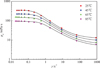 |
Fig. 3. Variation of slick-water viscosity against shear rate under different temperatures; symbols refer to measured data, while lines represent fitted results by Chang–Darby rheological model. |
As discussed in Section 2.2, the rheological parameters in Chang–Darby model are necessary to predict friction loss for polymer solution, so the Chang–Darby model was used to represent the viscosity-shear rate relationship at the whole shear region, which is defined as follows (Darby and Chang, 1984), and the fitted parameters together with other details of slick-water are summarized in Table 1. (17)where μ
a is the apparent viscosity, Pa·s; μ
∞ is the infinite shear rate viscosity, Pa·s.
(17)where μ
a is the apparent viscosity, Pa·s; μ
∞ is the infinite shear rate viscosity, Pa·s.
Properties of slick-water.
Additionally, for particles settling in slick-water, its viscoelasticity can significantly affect particle settling velocity. An integrated settling velocity model (Zhang et al., 2016) was used to accurately predict particle settling velocity in slick-water, which is as follows:![Mathematical equation: $$ {V}_{\mathrm{s}}=\mathrm{VF}{\left[\frac{g\left({\rho }_{\mathrm{p}}-{\rho }_{\mathrm{l}}\right){d}^{n+1}}{18K}\right]}^{\frac{1}{3n-1}} $$](/articles/ogst/full_html/2018/01/ogst180026/ogst180026-eq20.gif) (18)where, K is the consistency coefficient, Pa·s
n
; n is the flow behavior index and VF is the settling velocity factor, which is as follows:
(18)where, K is the consistency coefficient, Pa·s
n
; n is the flow behavior index and VF is the settling velocity factor, which is as follows:![Mathematical equation: $$ \mathrm{VF}=0.001{1}^{\frac{2n}{3n-1}}{\left[\frac{9\lambda \left(2{n}^2+n+1\right)}{K}\right]}^{\frac{1}{3n-1}} $$](/articles/ogst/full_html/2018/01/ogst180026/ogst180026-eq21.gif) (19)
(19)
3 Results and discussion
The nonlinear equation group is solved using a Global Search Algorithm in Matlab environment. Firstly, a stationary particle bed is assumed to be existence, if the maximum friction force between particle bed and pipe wall is exceeded, the particle bed starts to move, so the stationary particle bed changes to be a moving particle bed. In addition, if the height of moving particle bed is less than zero, the flow pattern turns into full suspension flow, which can be described by equation (10). Because few experiments have been conducted to study particle-fluid flow in a high inclined pipe, the experimental results for particle-fluid mixture transport in an approximate horizontal and horizontal pipe were used to validate the model and algorithm. Comparison between measured pressure gradient from Doron and Barnea (Doron et al., 1987, 1997) and predicted results from the two-layer transport model was carried out as shown in Figure 4. It is clear that the agreement between measured pressure gradient and predicted results is good, so it is no doubt that the downward flow of particle-fluid mixture through a curving pipe can be accurately described by the two-layer model. According to the modified two-layer model, the transport of particles carried by slick-water in a curving pipe is investigated. The flow pattern is observed and the variation of which against inclined angle is analyzed. The parameters used in numerical calculation are summarized in Table 2.
 |
Fig. 4. Comparison between measured pressure gradient and predicted results. |
Parameters used in numerical calculation.
3.1 Variation of flow pattern against inclined angle
The variation of mixture flow parameters against inclined angle is shown in Figure 5, and it is observed that the transport process can be divided into three stages. (1) When particle-fluid mixture just enters the curving segment (α < 15°), because the inclined angle is small, particles are still fully suspended into the carrier fluid. However, due to settling behavior of particles, they are inclined to accumulate near the pipe bottom, so the particle volumetric concentration decreases from pipe top to bottom, and a heterogeneous full suspension flow is observed. (2) As the increase in inclined angle (15° < α < 60°), particle settling in normal direction of a curving pipe increases, and some particles settle out of fluid and accumulate on pipe bottom. Therefore, a particle bed, which moves along the pipe, forms on the pipe bottom as shown in Figure 5d. At this stage, a full suspension layer is also observed above the particle bed, so a particle bed load flow pattern occurs. Because the height of particle bed is small, it moves almost at the same velocity as the upper suspension layer, the transport velocity of which is a little lower than the injected velocity. Because the tangential component of particle bed gravity has a strong contribution to its moving along pipe, so the transport velocity of particle bed increases with the increase in the height of particle bed. In addition, due to particle settling, the particle volumetric concentric of suspension layer dramatically decreases. Figure 6 shows the normal distribution of particle volumetric concentrations. It is clear that only a few of particles are suspended at the top of a pipe, and the particle volumetric concentration exponentially decreases from pipe top to bottom. Because particle normal settling strengths, the particle volumetric concentration decreases with the increase in inclined angle, while the height of particle bed increases. During this stage, the friction loss is composed of solid-fluid friction loss between suspension layer and pipe wall and solid-solid friction loss between moving particle bed and pipe wall, and because the height of particle bed is small, the solid-fluid friction loss has a main contribution. (3) For a high inclined angle (α > 60°), the normal component of particle gravity gradually increases, so the contribution of normal gravity component to particle settling changes to be larger than that of the tangential gravity component to flow along the pipe. Therefore, numerous particles settle out of fluid and accumulate on pipe bottom, and the height of particle bed dramatically increases. At this stage, the transport of particle bed is mainly induced by fluid drag, the friction loss between particle bed and pipe wall increases, and solid-solid friction loss overshadows solid-fluid friction loss. Therefore, solid-solid friction quickly increases with the increase in the height of particle bed, while its moving velocity sharply decreases. However, because the cross-sectional area of suspension layer decreases, the flow velocity of upper suspension layer also increases. It is clear from Figure 5c that the particle volumetric concentration decreases for small inclined angle, while it gradually increases with the increase in inclined angle because of high transport velocity of suspension layer, which exerts a strong lifting and drag force on particles on the surface of particle bed. However, a stationary particle bed has not been observed due to high transport velocity of suspension layer at an injected rate of 5 m/s.
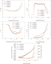 |
Fig. 5. Variation of mixture transport parameters against inclined angle under different particle densities: (a) transport velocity of suspension layer; (b) transport velocity of particle bed; (c) average particle volumetric concentration of suspension layer; (d) particle bed height; (e) pressure gradient. |
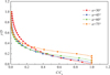 |
Fig. 6. Normal concentration distribution of particles in a curving pipe. |
3.2 Effect of slick-water rheological property
The rheological property of viscoelastic fluid can affect particle settling velocity and friction loss. As the decrease in consistency coefficient, particle settling velocity increases, so particles quickly settle out of carried fluid and accumulate on pipe bottom even at a smaller inclined angle as shown in Figure 7d. A particle bed load flow is earlier observed for carrier fluid with a smaller consistency coefficient, and the particle volumetric concentration is very sensitive to fluid rheological property as shown in Figure 7c. In stage 2, the contribution of particle settling to tangential flow is dominant, so the height of particle bed decreases with the decrease in fluid consistency coefficient, and this subsequently causes a small transport velocity of suspension layer and particle bed. In addition, the solid-fluid friction factor and friction loss decrease with the decrease in fluid consistency coefficient. However, for a large inclined angle at stage 3, the effect of particle normal settling starts to be dominant and solid-solid friction loss gradually governs the variation of pressure gradient. Therefore, the height of particle bed quickly increases with the decrease in fluid consistency coefficient, and this also causes the transport velocity of suspension layer to increase. In addition, because the friction factor is small for a small fluid consistency coefficient, the friction loss for the four fluids with different rheological properties is almost the same as shown in Figure 7e.
 |
Fig. 7. Variation of mixture transport parameters against inclined angle under different fluid rheological properties: (a) transport velocity of suspension layer; (b) transport velocity of particle bed; (c) average particle volumetric concentration of suspension layer; (d) particle bed height; (e) pressure gradient. |
3.3 Effect of particle size
Since the viscosity of slick-water is low, its ability to transport proppant particles is poor. When slick-water is used in hydraulic fracturing to develop shale gas and tight oil, fine proppant particles are commonly applied. Because small particles can be carried deep into a hydraulic fracture, the placement of proppant particles is significantly improved, and this greatly increases the fracture conductivity. Figure 8 shows the variation of transport parameters against inclined angle under different particle diameters. Due to high settling velocity of large particles, they can quickly settle out of carried fluid and accumulate on pipe bottom to form a particle bed. It is clear from Figure 8d that a particle bed load flow can be observed at a smaller inclined angle for large particles and the transition angle between full suspension flow and particle bed load flow reduces with the increase in particle size. On the contrary, small particles can be well transported by carrier fluid, so the particles with the diameter of 0.25 mm always keep suspended during transport through the whole curing pipe.
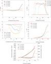 |
Fig. 8. Variation of mixture transport parameters against inclined angle under different particle diameters: (a) transport velocity of suspension layer; (b) transport velocity of particle bed; (c) average particle volumetric concentration of suspension layer; (d) particle bed height; (e) pressure gradient. |
It is also observed from Figure 8d that, the height of particle bed doesn’t linearly increase with the increase in particle diameter. The reason is that the major transport behavior of small particles is governed by the drag of carrier fluid, so a small particle bed forms. Therefore, for small particles with small settling velocity in stage 2, their hydrodynamic performance is governed by the drag of carried fluid, and the height of particle bed reduces with the decrease in particle diameter. However, the settling behavior is dominant for large particles and has a significant contribution to tangential transport, so the tangential transport of large particles strengths and a small particle bed forms. In addition, particle normal settling increases with the increase in particle diameter in stage 3, so the height of particle bed quickly increases, and the transport velocity of particle bed is high due to the drag of carrier fluid, which also has a high flow velocity.
3.4 Effect of particle injected volumetric concentration
Figure 9 shows the variation of mixture transport parameters against inclined angle under different particle injected volumetric concentration. It is clear that more particles settle out of fluid and accumulate on pipe bottom for high particle injected concentration, so a particle bed load flow occurs at a smaller inclined angle. However, the height of particle bed is almost the same for different injected concentration in stage 2. Since the suspension layer of particle-fluid mixture is treated as pseudo-fluid, its density increases with the increase in particle injected concentration, so the solid-fluid friction loss increases and this decreases the transport velocity of suspension layer. Therefore, the average particle volumetric concentration of suspension layer and transport velocity of particle bed decrease with the increase in injected concentration, as shown in Figures 9b and 9c, and this subsequently reduces the solid-solid friction loss between particle bed and pipe wall. When the transport of particle-fluid mixture enters stage 3 at a high inclined angle, particle normal settling starts to be dominant, and the height of particle bed dramatically increases. More particles settle out of fluid and accumulate on pipe bottom with the increase in injected concentration, so a large particle bed forms for a high injected concentration. This reduces the cross-sectional area of suspension layer, causing a high transport velocity. In addition, because the drag of carrier fluid on particle bed totally overshadows the solid-solid friction between particle bed and pipe wall, although the height of particle bed increase, its transport velocity still increases with the increase in injected velocity. Since the pressure gradient is mainly governed by solid-solid friction loss, the pressure gradient also increases with the increase in injected particle volumetric concentration.
 |
Fig. 9. Variation of mixture transport parameters against inclined angle under different particle injected volumetric concentrations: (a) transport velocity of suspension layer; (b) transport velocity of particle bed; (c) average particle volumetric concentration of suspension layer; (d) particle bed height; (e) pressure gradient. |
3.5 Effect of injected rate
Since the drag of carried fluid on particles and particle turbulent diffusion in carried fluid depends on fluid flow velocity, the injected rate can significantly affect the flow pattern of particle-fluid mixture in a curving pipe. The effect of injected velocity on particle-fluid mixture transport is investigated in this section, and the results are shown in Figure 10. It is clear that a small injected rate causes a small transport velocity of suspension layer, which exerts a small drag force and lifting force, so a particle bed load flow occurs at a small inclined angle. Since the centrifugal force of transporting particles increases with the increase in injected rate, in stage 2, particles are more inclined to settle out of carried fluid and accumulate on pipe wall to form a bed at a high injected rate. Because the height of particle bed increases with the increase in inclined angle, the transport velocity of suspension layer also increases, which exerts larger drag force on particles. When the drag force totally overshadows the centrifugal force in stage 3, more particles on the top surface of particle bed are re-suspended into suspension layer, so the height of particle bed decreases. In addition, because particle carried ability of fluid and friction loss is proportion to injected rate, the average particle volumetric concentration of suspension layer, transport velocity of particle bed and pressure gradient increase with the increase in injected rate.
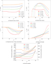 |
Fig. 10. Variation of mixture transport parameters against inclined angle under different injected rates: (a) transport velocity of suspension layer; (b) transport velocity of particle bed; (c) average particle volumetric concentration of suspension layer; (d) particle bed height; (e) pressure gradient. |
3.6 Flow pattern map
As analyzed above, when particle-fluid mixture transport through a curving pipe, a particle bed load flow can be observed, but due to the injected rate is high, the particle bed keeps moving and no stationary particle bed occurs. During hydraulic fracturing, since the friction loss sharply increases with the increase in the height of particle bed, a particle bed load flow can cause extra energy loss. In addition, a moving particle bed also can severely abrade fracturing pipes, and this may cause safety accidents. Therefore, a particle bed load flow in the pipe should be avoided in hydraulic fracturing.
In this section, numerous calculations have been carried out under different injected rates, the critical transition velocities between different stages were investigated, and a flow pattern map of particle-fluid transport in a curving pipe was established as shown in Figure 11. It is clear that the critical transition velocity quickly increases with the increase in inclined angle for the injected rates less than 1 m/s, while the critical transition velocity almost keeps constant in stage 3. In stage 2, as the injected velocity increases, particles in particle bed are gradually re-suspended into suspension layer, so a particle bed load flow changes to be a full suspension flow when the injected rate is higher than lower critical transition velocity. However, a centrifugal effect region occurs in this stage, for a high injected rate (>1 m/s), particle centrifugal force increases with the increase in injected rate, which causes particles to be inclined to accumulate near pipe bottom, so a particle bed re-forms with the increase in injected rate, and a full suspension flow reversely turns into a particle bed load flow. Subsequently, when the injected rate is bigger than upper critical transition velocity, the drag of carrier fluid totally overshadows the centrifugal force effect, so the flow pattern turns into full suspension flow again. It is observed from Figure 11 that the maximum critical transition velocity occurs at an inclined angle of 90°, where the flow turns from a curving pipe to a horizontal pipe. Therefore, in order to safely and efficiently execute hydraulic fracturing treatments, the applied injected rate must be higher than the maximum critical transition velocity to avoid a particle bed load flow.
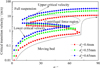 |
Fig. 11. Flow pattern map for particle-fluid mixture transport in a curving pipe. |
4 Conclusion
In this work, a two-layer model was used to model aslant downward transport of proppant particles driven by slick-water in a curving pipe. The viscoelastic properties of carrier fluid were taken into consideration, based on which a friction factor correlation and settling velocity model were applied to modify the two-layer model. In addition, an energy equation was established to determine fluid temperature to accurately characterize its rheological properties. The model is solved using a Global Search Algorithm in Matlab environment, the variation of flow pattern was investigated, and a flow pattern map was established. When particles load fluid just enters a curving pipe with a small inclined angle (α < 15°), particles keep full suspended in the carrier fluid. Subsequently, for a large inclined angle (15° < α < 60°), particles settle out of carrier fluid and accumulate on pipe bottom to form a particle bed, which keeps moving, so a particle bed load flow occurs. In this stage, since the height of a particle bed is small, it transports at a high velocity. Then particles quickly settle out of carrier fluid at approximately horizontal flow (60° < α < 9°), so a particle bed quickly develops while its transport velocity sharply decreases. The flow pattern of particle-fluid mixture in a curving pipe changes from particle bed load flow to full suspension flow with the increase in injected rate, and the transition velocity increases with the increase in inclined angle. However, an inverse transition occurs due to the effect of centrifugal force at intermediate inclined angle, where a full suspension flow inversely turns into a particle bed load flow with the increase in injected rate. Ultimately, in order to safely and efficiently execute hydraulic fracturing treatments in a horizontal well, a minimum injected rate of proppant load fracturing fluid must be kept in mind, which can be determined by the two-layer transport model.
Acknowledgments
This study was supported by the Natural Science Foundation of Shandong Province, China (ZR2018BEE005) and Doctoral Fund of Qingdao University of Science and Technology (0100229017).
References
- Arthur J.D., Bohm B., Coughlin B.J., Layne M. (2009) Evaluating implications of hydraulic fracturing in shale-gas reservoirs, J. Petrol. Technol. 61, 8, 53–54. [Google Scholar]
- Bird R.B. (1987) Dynamics of polymeric liquids, Wiley, New York. [Google Scholar]
- Brown M.L., Ozkan E., Raghavan R.S., Kazemi H. (2011) Practical solutions for pressure-transient responses of fractured horizontal wells in unconventional shale reservoirs, SPE Reserv. Eval. Eng. 14, 6, 663–676. [CrossRef] [Google Scholar]
- Chang H.D. (1982) Correlation of turbulent drag reduction in dilute polymer solutions with rheological properties by an energy dissipation model, PhD Thesis, Texas A & M University, Texas. [Google Scholar]
- Chen N.H. (1979) An explicit equation for friction factor in pipe, Ind. Eng. Chem. Fundamen. 18, 3, 296–297. [Google Scholar]
- Cho H., Shah S.N., Osisanya S.O. (2002) A three-segment hydraulic model for cuttings transport in coiled tubing horizontal and deviated drilling, J. Can. Petrol. Technol. 41, 6, 32–39. [Google Scholar]
- Darby R., Chang H.D. (1984) Generalized correlation for friction loss in drag reducing polymer solutions, Aiche J. 30, 2, 274–280. [CrossRef] [Google Scholar]
- Doron P., Barnea D. (1993) A three-layer model for solid-liquid flow in horizontal pipes, Int. J. Multiphas. Flow 19, 6, 1029–1043. [CrossRef] [Google Scholar]
- Doron P., Barnea D. (1995) Pressure drop and limit deposit velocity for solid-liquid flow in pipes, Chem. Eng. Sci. 50, 10, 1595–1604. [CrossRef] [Google Scholar]
- Doron P., Granica D., Barnea D. (1987) Slurry flow in horizontal pipes – experimental and modeling, Int. J. Multiphas. Flow 13, 4, 535–547. [CrossRef] [Google Scholar]
- Doron P., Simkhis M., Barnea D. (1997) Flow of solid-liquid mixtures in inclined pipes, Int. J. Multiphas. Flow 23, 2, 313–323. [Google Scholar]
- Gallego F., Shah S.N. (2009) Friction pressure correlations for turbulent flow of drag reducing polymer solutions in straight and coiled tubing, J. Petrol. Sci. Eng. 65, 3–4, 147–161. [CrossRef] [Google Scholar]
- Matoušek V. (2009) Predictive model for frictional pressure drop in settling-slurry pipe with stationary deposit, Powder Technol. 192, 3, 367–374. [CrossRef] [Google Scholar]
- Marfaing O., Guingo M., Laviéville J.M., Mimouni S. (2017) Analytical void fraction profile near the walls in low Reynolds number bubbly flows in pipes: experimental comparison and estimate of the dispersion coefficient, Oil Gas Sci. Technol. - Rev. IFP Energies nouvelles 72, 4. [CrossRef] [Google Scholar]
- Noetinger B. (1989) A two fluid model for sedimentation phenomena, Physica A 157, 1139–1179. [CrossRef] [Google Scholar]
- Palisch T.T., Vincent M.C., Handren P.J. (2010) Slickwater fracturing: food for thought, SPE Prod. Oper. 25, 3, 327–344. [Google Scholar]
- Pearson J.R.A. (1994) On suspension transport in a fracture: framework for a global model, J. Non-Newton. Fluid 54, 6, 503–513. [CrossRef] [Google Scholar]
- Różański J. (2011) Flow of drag-reducing surfactant solutions in rough pipes, J. Non-Newton. Fluid 166, 5, 279–288. [CrossRef] [Google Scholar]
- Ramadan A., Skalle P., Saasen A. (2005) Application of a three-layer modeling approach for solids transport in horizontal and inclined channels, Chem. Eng. Sci. 60, 10, 2557–2570. [CrossRef] [Google Scholar]
- Ravelet F., Bakir F., Khelladi S., Rey R. (2013) Experimental study of hydraulic transport of large particles in horizontal pipes, Exp. Therm. Fluid Sci. 45, 2, 187–197. [CrossRef] [Google Scholar]
- Ribeiro J.M., Eler F.M., Martins A.L., Scheid C.M., Calçada L.A., Meleiro L.A.D.C. (2017) A simplified model applied to the barite sag and fluid flow in drilling muds: simulation and experimental results, Oil Gas Sci. Technol. - Rev. IFP Energies nouvelles 72, 23. [Google Scholar]
- Roussel N.P., Sharma M.M. (2011) Optimizing fracture spacing and sequencing in horizontal-well fracturing, SPE Prod. Oper. 26, 2, 173–184. [Google Scholar]
- Sovacool B.K. (2014) Cornucopia or curse? Reviewing the costs and benefits of shale gas hydraulic fracturing (fracking), Renew. Sust. Energ. Rev. 37, 3, 249–264. [CrossRef] [Google Scholar]
- Toms B.A. (1948) Some observations on the flow of linear polymer solutions through straight tubes at large Reynolds numbers, in: G.W. Scott Blair (ed.), Proc. First International Congress on Rheology, The Netherlands. [Google Scholar]
- Zhang G., Gutierrez M., Li M. (2017) A coupled CFD-DEM approach to model particle-fluid mixture transport between two parallel plates to improve understanding of proppant micromechanics in hydraulic fractures, Powder Technol. 308, 235–248. [CrossRef] [Google Scholar]
- Zhang G., Li M., Geng K., Han R., Xie M., Liao K. (2016) New integrated model of the settling velocity of proppants falling in viscoelastic slick-water fracturing fluids, J. Nat. Gas Sci. Eng. 33, 518–526. [CrossRef] [Google Scholar]
- Zou C., Dong D., Wang Y., Li X., Huang J., Wang S., Guan Q., Zhang C., Wang H., Liu H. (2015) Shale gas in China: characteristics, challenges and prospects(I), Petrol. Explor. Deve. 42, 6, 753–767. [CrossRef] [Google Scholar]
All Tables
All Figures
|
Fig. 1. Schematic of a hydraulic fracturing in a horizontal well. |
| In the text | |
|
Fig. 2. Geometric schematic of two-layer particle-fluid mixture flow. |
| In the text | |
|
Fig. 3. Variation of slick-water viscosity against shear rate under different temperatures; symbols refer to measured data, while lines represent fitted results by Chang–Darby rheological model. |
| In the text | |
|
Fig. 4. Comparison between measured pressure gradient and predicted results. |
| In the text | |
|
Fig. 5. Variation of mixture transport parameters against inclined angle under different particle densities: (a) transport velocity of suspension layer; (b) transport velocity of particle bed; (c) average particle volumetric concentration of suspension layer; (d) particle bed height; (e) pressure gradient. |
| In the text | |
|
Fig. 6. Normal concentration distribution of particles in a curving pipe. |
| In the text | |
|
Fig. 7. Variation of mixture transport parameters against inclined angle under different fluid rheological properties: (a) transport velocity of suspension layer; (b) transport velocity of particle bed; (c) average particle volumetric concentration of suspension layer; (d) particle bed height; (e) pressure gradient. |
| In the text | |
|
Fig. 8. Variation of mixture transport parameters against inclined angle under different particle diameters: (a) transport velocity of suspension layer; (b) transport velocity of particle bed; (c) average particle volumetric concentration of suspension layer; (d) particle bed height; (e) pressure gradient. |
| In the text | |
|
Fig. 9. Variation of mixture transport parameters against inclined angle under different particle injected volumetric concentrations: (a) transport velocity of suspension layer; (b) transport velocity of particle bed; (c) average particle volumetric concentration of suspension layer; (d) particle bed height; (e) pressure gradient. |
| In the text | |
|
Fig. 10. Variation of mixture transport parameters against inclined angle under different injected rates: (a) transport velocity of suspension layer; (b) transport velocity of particle bed; (c) average particle volumetric concentration of suspension layer; (d) particle bed height; (e) pressure gradient. |
| In the text | |
|
Fig. 11. Flow pattern map for particle-fluid mixture transport in a curving pipe. |
| In the text | |