Regular Article
The Theis solution for subdiffusive flow in rocks
1
R. Raghavan, Inc., P.O. Box 52756, Tulsa, OK 74152, USA
2
Kappa Engineering, 11767 Katy Freeway, #500, Houston, TX 77079, USA
* Corresponding author: This email address is being protected from spambots. You need JavaScript enabled to view it.
Received:
23
August
2018
Accepted:
22
October
2018
Abstract
The central contribution of this work is the development of a “master” solution similar to the Theis solution to evaluate well responses under subdiffusive flow. Models based on subdiffusion employ fractional constitutive laws, a redefinition of Darcy’s law. Subdiffusive models discussed here are particularly useful to address situations where the internal architecture of the geological medium, such as fluvial and fractured systems, matters and where the existence of topological, geometrical and spatial influences result in distorted flow paths and a loss in connectivity. The developed solution provides the means for addressing these ends.
© R. Raghavan & C. Chen, published by IFP Energies nouvelles, 2019
 This is an Open Access article distributed under the terms of the Creative Commons Attribution License (http://creativecommons.org/licenses/by/4.0), which permits unrestricted use, distribution, and reproduction in any medium, provided the original work is properly cited.
Nomenclature
c : Compressibility (LT2/M)
C : Unit storage factor (ML2/T2)
d : Distance (Ln, n = 1, 2 or 3)
df : Hausdorff dimension
d w : Anomalous diffusion coefficient (random walk dimension)
 :
Caputo operator
:
Caputo operator
 :
Function to incorporate naturally fractured reservoir formulation
:
Function to incorporate naturally fractured reservoir formulation
h : Thickness [L]
![Mathematical equation: $ {H}_{p,q}^{m,n}[x{|}_{({b}_1,{B}_1),...,({b}_q,{B}_q)}^{({a}_1,{A}_1),...,({a}_p,{A}_p)}]$](/articles/ogst/full_html/2019/01/ogst180275/ogst180275-eq3.gif) :
Fox function
:
Fox function
Kν (z): Modified Bessel function; second kind of order ν
k : Permeability [L2]
 :
See equation (2)
:
See equation (2)
Lf : One-half the length of hydraulic fracture [L]
 :
Reference length [L]
:
Reference length [L]
p : Pressure [M/L/T2]
q : Rate [L3/T]
 :
Real part of a number
:
Real part of a number
r : Distance [L]
t : Time [T]
s : Laplace variable [1/T]
 :
Skin factor
:
Skin factor
S : Skin factor of Hawkins
x,y : Coordinates [L]
z : A complex function
α : Exponent; see equation (1)
Γ(⋅): Gamma function
γ : Euler’s constant (0.5772…)
η : Diffusivity; various
 :
“Diffusivity”; see equation (7) [L2/Tα]
:
“Diffusivity”; see equation (7) [L2/Tα]
θ : scaling variable; see equation (34)
λ : Mobility [L T/M]
μ : Viscosity [M/L/T]
ϕ : Porosity [L3/L3]
ψ(x): Digamma function
Subscripts
D: Dimensionless
f: Hydraulic fracture
i: Initial
sf: Sandface
t: Total
u: Unit well
w: Well, wellbore
Superscripts
–: Laplace transform
1 Introduction
Forecasts, assessments and evaluations of subsurface resources whether they be hydrocarbon production or geothermal extraction (Arps, 1945; Fetkovich, 1980; Whiting and Ramey, 1969), sequestration and waste disposal technologies (Bodvarsson et al. 1999; IPCC, 2005) or groundwater systems require discernment of flow and transport mechanisms. The Theis (1935) solution has been the linchpin to assess the flow properties of the reservoir rock (aquifer). Both its adequacy and its limits have been of interest and tested over the years by statistical techniques because it ignores the influence of spatial variability within its support volume (Romeu and Noetinger, 1995; Sanchez-Vila et al., 2006; Schad and Teutsch, 1994; Warren and Price, 1961). Ignoring internal architecture, geologic structure and internal imprint such as stratification, intercalations and barriers that produce distorted flow paths, however, results in a serious underestimation of the resource (Raghavan, 2004, 2009b; Thomas et al., 2005). Other approaches that account for spatial variability have represented transient diffusion by representing the porous medium as a fractal object (Camacho-Velázquez et al., 2008; Chang and Yortsos, 1990; Raghavan, 2009a). This approach is particularly fruitful because it has been suggested (Kim et al., 2015; Raghavan, 2011) and shown (Benson et al., 2004; Chu et al., 2017, 2018) that there is an interdependence between the topological and geometric properties of the reservoir rock and the physics of fluid movement particulary if the geology is complex. This hypothesis leads to the consideration that diffusion is anomalous and a reconsideration of Darcy’s law; see for example, Nigmatullin (1984, 1986), Le Mẽhautẽ (1984), Dassas and Duby (1995), Henry et al. (2010) to name a few of the many such citations. Anomalous diffusion implies a nonlinear scaling of the mean square displacement of the transient front with time. Well responses often display power-law behavior (Chang and Yortsos, 1990; Raghavan and Chen, 2013a).
The goal of this study is to explore the development and application of interference tests for subdiffusive flows. The first step involves examination of the Theis (1935) solution for subdiffusive flow. Although such a solution has been available for some time, the solution is rarely recognized probably because it was presented as an aside to the study of fractured wells (Raghavan, 2012). We flesh out the details of the solution as they are not yet available and more importantly present a correlation in the manner of Theis (1935) as a “working” solution. In addition, we examine new developments that have appeared in the literature and indicate adjustments that need to be made if the goal is to model subdiffusive flow (Su et al., 2015). We then examine pressure distributions by injecting through a vertical fracture along the lines proposed in Uraiet et al. (1977) as the active (pumping) well is often stimulated by a vertical fracture.
The model discussed in this work is a viable option to evaluate well tests in fluvial (and fractured) systems that display near power-law behaviors; indeed, they avoid conjuring up geological options where we would tend to look askance at analyses.
2 Problem statement
We proceed in the usual way by considering the flow of a slightly compressible fluid of compressibility, c, and viscosity, μ, to a well of radius, rw, located at the origin of a reservoir of constant thickness, h, that is at initial pressure, pi, and infinite in its areal extent. The well center is taken to be the origin and the fluid properties are assumed to be constant. Again, as usual, we formulate the problem by combining the conservation equation, the flux law for subdiffusive flow and the equation of state for a slightly compressible fluid. The solution is developed in terms of the Laplace transformation in the cylindrical coordinate system presuming symmetry under the assumptions that the well penetrates the reservoir completely and is produced (pumped) at a constant rate, q. Thus, except for the flux law, a fractional form of Darcy’s law, we consider the standard problem. We work in terms of the Laplace transformation and denote the Laplace variable by the symbol, s. As a result, the ideas of Warren and Root (1963) or de Swaan-O (1976) for naturally fractured reservoirs may be incorporated in the formulations that follow through a kernel,  , in the arguments of the Bessel functions; see Noetinger and Estebenet (2000), Noetinger et al. (2001, 2016), Albinali et al. (2016) and Raghavan and Chen (2017) for illustrations that incorporate subdiffusive mechanisms in the matrix system and in the fracture system if needed, and for the definition of
  . Another direct benefit is the option to include the wellbore storage effect (see Appendix).
Over the past few years, particularly since 2011, a number of articles pertaining to the behavior of wells in subdiffusive systems has appeared in the literature, and different choices have been made with respect to the development of the mathematical model. The choices made in this work are dictated by our experiences in working on shale reservoirs and the need to address reserves and forecast performance. A comprehensive discussion of the choices may be found in Raghavan and Chen (2013a) where we discuss modifications to Beier’s (1994) model.
2.1 The Darcy law
In our opinion, one of the best expositions of the flux law for subdiffusive flow is the one given in Henry et al. (2010). They show that for subdiffusive flows the velocity, v(x,t), at a location, x, at time, t, is given by![Mathematical equation: $$ v({x},t)=-\stackrel{\tilde }{\lambda }\frac{{\mathrm{\partial }}^{1-\alpha }}{\mathrm{\partial }{t}^{1-\alpha }}\left[\nabla p({x},t)\right], $$](/articles/ogst/full_html/2019/01/ogst180275/ogst180275-eq11.gif) (1)where the symbol, p(x,t) is the pressure at a point in time, and
(1)where the symbol, p(x,t) is the pressure at a point in time, and (2)
(2)
The fractional derivative, ∂α f(t)/∂tα, for 0<α<1 used in the Caputo (1967) sense is given by (3)where Γ(⋅) is the Gamma function. For α = 1, equation (1) reverts to the classical Darcy equation. For reservoir rocks, to our knowledge, only the recent study by Raghavan and Chen (2018) has directly addressed estimates of α; for shales in the Permian basin they report the following estimates: 0.56 ≤ αf ≤ 0.91 and 0.77 ≤ αm ≤ 0.94, where the subscripts “f” and “m” stand for the fissure and matrix systems, respectively. Estimates of α may also be deduced from other works using the guidelines in Beier (1990) and Metzler et al. (1994). Values in the range 0.6 < α < 0.86 are reported in Acuna et al. (1995), while Flamenco-Lopez and Camacho-Velázquez (2001) report that α was in the range 0.47 < α < 0.67. Also from Le Borgne et al. (2004, 2007), we obtain α to be 0.71.
The Laplace transformation of the Caputo fractional operator,  , is given by
 (4)
(4)
This expression in equation (1) implies that the flux at time, t, may not be obtained directly from the instantaneous pressure distribution, p(x,t).
2.2 Formulation
Considering cylindrical coordinates and assuming the well axis passes through the origin, the application of the conservation of mass principle to a control volume for a slightly compressible fluid yields (5)where ϕ is the porosity of the medium, and r is the distance from the well center. On substituting the right-hand side of equation (1) for v(r,t) and integrating, we obtain the partial differential equation for transient diffusion under subdiffusive flow to be
 (6)where
  , the “diffusivity” of the medium, is given as
 (7)
(7)
We seek a solution to equation (6) subject to the following initial and boundary conditions: (8)
(8) (9)and
![Mathematical equation: $$ {\left[r\frac{{\mathrm{\partial }}^{1-\alpha }}{\mathrm{\partial }{t}^{1-\alpha }}\left(\frac{\mathrm{\partial }p}{\mathrm{\partial }r}\right)\right]}_{{r}_{\mathrm{w}}}=\frac{{q\mu }}{2\pi \mathop{k}\limits^\tildeh},\enspace \hspace{1em}t>0. $$](/articles/ogst/full_html/2019/01/ogst180275/ogst180275-eq22.gif) (10)
(10)
Equation (10) specifies the condition for a well of finite radius, rw. The Theis solution, however, requires that we determine the solution when the well radius is vanishingly small; that is, a line source or the solution as  . As the finite well-radius solution is more general, we consider this general solution first and then extract the solution corresponding to a well that is a line-source.
3 General solution
The procedure for obtaining the solution we desire is straightforward and may be found in many texts. Working in terms of the pressure difference, Δp (r,t) [pi−p (r,t)], with respect to the initial pressure, pi, and denoting  to be the Laplace transform of Δp, the Laplace transform of equation (6) becomes a modified Bessel equation of order 0, the general solution of which is
 (11)with I0 (x) and K0 (x) representing the modified Bessel functions of the first and second kind of order 0, respectively, and
 (12)
(12)
If the outer-boundary condition given by equation (9) is to be satisfied, then B = 0, because I0 (x) → ∞ as x → ∞. Application of the Laplace transform to equation (10) and further simplification provides the constant A; thus, the pressure distribution is (13)
(13)
3.1 Solutions for the situation xK1 (x) as x → 0
This approximation leads to the consideration of solutions for two important situations. First, if we consider long enough times, then the approximation provides the long-time response for a well of radius, rw; second, if we were to consider situations where rw → 0, then the approximation provides the solution for a line-source well, and the analog of the Theis (1935) solution for subdiffusive flow is obtained. These observations also suggest that at long enough times the line-source solution becomes asymptotic to the finite-well-radius solution similar to the classical case; see Mueller and Witherspoon (1965). Because xK1 (x) → 1 as x → 0, the expression for the pressure distribution around a line-source well under subdiffusion turns out to be (14)
(14)
Saxena et al. (2006) show that![Mathematical equation: $$ 2{L}^{-1}[{s}^{-\varrho }{K}_{\nu }(z{s}^{\varsigma })]={t}^{\varrho -1}{H}_{\mathrm{1,2}}^{\mathrm{2,0}}\left[\frac{{z}^2{t}^{-2\varsigma }}{4}{|}_{\left(\frac{\nu }{2},1\right),\left(-\frac{\nu }{2},1\right)}^{\varrho,2\varsigma }\right], $$](/articles/ogst/full_html/2019/01/ogst180275/ogst180275-eq29.gif) (15)where the symbol
(15)where the symbol ![Mathematical equation: $ {H}_{p,q}^{m,n}[x{|}_{({b}_1,{B}_1),...,({b}_q,{B}_q)}^{({a}_1,{A}_1),...,({a}_p,{A}_p)}]$](/articles/ogst/full_html/2019/01/ogst180275/ogst180275-eq30.gif) is the Fox function or the H-function,
is the Fox function or the H-function,  ,
,  ,
,  . To our knowledge, the Fox function is best computed with the aid of packages such as Mathematica; see Weisstein (2018); see also Mainardi et al. (2005). The simplest alternative to compute Δp(r,t) is by inverting the expression in equation (13) by the Stehfest algorithm (1970a, b).
On defining dimensionless variables corresponding to distance, rD, time, tD, and pressure, pD (rD,tD), respectively, by (16)
(16) (17)and
 (18)we obtain
![Mathematical equation: $$ {p}_{\mathrm{D}}({r}_{\mathrm{D}},{t}_{\mathrm{D}})=\frac{1}{2}{t}_{\mathrm{D}}^{\frac{1-\alpha }{\alpha }}{H}_{\mathrm{1,2}}^{\mathrm{2,0}}\left[\frac{{r}_{\mathrm{D}}^2}{4{t}_{\mathrm{D}}}{|}_{(\mathrm{0,1}),(\mathrm{0,1})}^{2-\alpha,\alpha }\right]. $$](/articles/ogst/full_html/2019/01/ogst180275/ogst180275-eq37.gif) (19)
(19)
As noted earlier, an expression identical to that in equation (19) derived by the method of sources and sinks is given in Raghavan (2012) but the details we are about to discuss were not considered, as the goal there was to discuss the performance of fractured wells. First and foremost we should note that for α = 1, equation (19) does reduce to the Theis (1935) solution (20)where −Ei(−u) is the Exponential Integral and
  . Second, it is important to recognize that the time term in the coefficient of the Fox function arises out of the fractional Darcy law, equation (10), much in the same way as the exponent α on the right hand side of equation (6) arises in our development. There are many studies where the fractional form of Darcy’s law is not used (Atangana and Bildik, 2013), and solutions are presented using equation (6) with the classical definition of Darcy’s law; we are yet to understand the physics behind such approaches to study fluid movement in heterogeneous environments for it is not obvious as to how one may arrive at the differential equation of the form used here without the use a fractional form of Darcy’s law (or some other similar consideration). Third and most importantly, the expression on the right hand side of equation (19) suggests that a working solution for analyzing responses under subdiffusive flow may be obtained by plotting
  vs
vs  with ν = 2(1−α)/(α); this aspect is considered in Section 3.2 on Computational Results. This observation may be advantageous if measurements at several wells are addressed simultaneously during an interference test.
3.1.1 An asymptotic solution of equation (13)
Considering s → 0, and using the result that for small values of x, K0 (x) is given by (Carslaw and Jaeger, 1959)![Mathematical equation: $$ {K}_0(z)=-\left(\mathrm{ln}\frac{z}{2}+\gamma \right)+\frac{{z}^2}{4}\left[1-\left(\gamma +\mathrm{ln}\frac{z}{2}\right)\right]+O({z}^4\mathrm{ln}\enspace z), $$](/articles/ogst/full_html/2019/01/ogst180275/ogst180275-eq42.gif) (21)where γ is Euler’s constant, then after ignoring all but the first two terms on the right-hand side of equation (21), we may readily show from that the long-term approximation of equation (14) (or the long-time approximation of equation (13)) is
(21)where γ is Euler’s constant, then after ignoring all but the first two terms on the right-hand side of equation (21), we may readily show from that the long-term approximation of equation (14) (or the long-time approximation of equation (13)) is![Mathematical equation: $$ {p}_{\mathrm{D}}({r}_{\mathrm{D}},{t}_{\mathrm{D}})=\frac{1}{2}\frac{1}{\mathrm{\Gamma }(2-\alpha )}{t}_{\mathrm{D}}^{\frac{1-\alpha }{\alpha }}\left[\mathrm{ln}\frac{4{t}_{\mathrm{D}}}{{e}^{2\gamma }{r}_{\mathrm{D}}^2}-{\alpha \psi }(2-\alpha )\right], $$](/articles/ogst/full_html/2019/01/ogst180275/ogst180275-eq43.gif) (22)where ψ(⋅) is the Digamma function. The logarithmic derivative of pD (rD,tD) corresponding to equation (22) is, of course, given by
(22)where ψ(⋅) is the Digamma function. The logarithmic derivative of pD (rD,tD) corresponding to equation (22) is, of course, given by![Mathematical equation: $$ {{p}^{\prime}_{\mathrm{D}}\left({r}_{\mathrm{D}},{t}_{\mathrm{D}}\right)=\frac{1}{2}\frac{1}{\mathrm{\Gamma }\left(2-\alpha \right)}{t}_{\mathrm{D}}^{\frac{1-\alpha }{\alpha }}\left\{\left(1-\alpha \right)\left[\mathrm{ln}\frac{4{t}_{\mathrm{D}}}{{e}^{2\gamma }{r}_{\mathrm{D}}^2}-{\alpha \psi }\left(2-\alpha \right)\right]+\alpha \right\}. $$](/articles/ogst/full_html/2019/01/ogst180275/ogst180275-eq44.gif) (23)
(23)
Again for α = 1, this result corresponds to the semi-logarithmic approximation of the Theis (1935) solution, namely the Cooper and Jacob (1946) approximation. As we discuss below in a number of situations, like that discussed in Thomas et al. (2005), active well responses follow near power-law trends similar to those suggested by equation (23).
3.1.2 The instantaneous, line-source solution corresponding to equation (14)
Using the ideas in Carslaw and Jaeger (1959) it is rather easy to obtain the expression for the pressure distribution,  , at a point, (x,y), caused by an instantaneous, line-source at t = 0 located at the point (xi,yi). The expression is
![Mathematical equation: $$ \overline{\zeta }(x,y)=\frac{{s}^{\alpha -1}}{2\pi \stackrel{\tilde }{\eta }}{K}_0\left[{s}^{\frac{\alpha }{2}}{\left\{\frac{(x-{x}_i^\mathrm{\prime}{)}^2+(y-{y}_i^\mathrm{\prime}{)}^2}{\stackrel{\tilde }{\eta }}\right\}}^{\frac{1}{2}}\right]. $$](/articles/ogst/full_html/2019/01/ogst180275/ogst180275-eq46.gif) (24)
(24)
The three dimensional version of equation (24) may be found in Mendes et al. (2005). The line-source or point-source solution is particularly convenient for determining the nonlinear scaling of the space-time behavior of the transient front with the second moment, <r2>, of the transient scaling in the form (25)
(25)
For purposes of understanding well behavior, point- or line-source solutions are particularly convenient for developing pressure distributions in reservoirs produced through complex wellbores; see, for example, Raghavan and Ozkan (1994).
3.1.3 Vertically-fractured wells
The solution for a vertically fractured well may be obtained by suitably integrating the right-hand side of equation (24). Assuming the center of the fracture is at (xw,yw) and that the fracture extends from (xw−Lf) to (xw + Lf) with its plane parallel to y = 0, the pressure distribution in terms of the Laplace transformation is![Mathematical equation: $$ \overline{\Delta p}({x}_{\mathrm{D}},{y}_{\mathrm{D}})=\frac{\mu \mathcal{l}}{2\pi {k}_{\alpha }}{s}^{\alpha -1}{\int }_{-{L}_{\mathrm{f}}/\mathcal{l}}^{+{L}_{\mathrm{f}}/\mathcal{l}} \mathrm{d}{\lambda }\enspace \overline{\mathop{q}\limits^\tilde}\left({\widehat{x}}_{\mathrm{D}}\right){K}_0\left[\sqrt{u}\enspace \sqrt{(x-{\widehat{x}}_{\mathrm{w}}{)}_{\mathrm{D}}^2+{\left(y-{y}_{\mathrm{w}}\right)}_{\mathrm{D}}^2}\right], $$](/articles/ogst/full_html/2019/01/ogst180275/ogst180275-eq48.gif) (26)with
(26)with  being the reference length,
  being the flux distribution, and
  defined by
 (27)
(27)
In the following we consider the uniform-flux solutions; that is,  is independent of x and t. If this were the case, then equation (26) becomes
![Mathematical equation: $$ \begin{array}{ll}{\bar{p}}_{\mathrm{D}}({x}_{\mathrm{D}},{y}_{\mathrm{D}})& =\frac{\mathcal{l}}{2{L}_{\mathrm{f}}}{\left(\frac{\stackrel{\tilde }{\eta }}{{L}_{\mathrm{f}}^2}\right)}^{\frac{1-\alpha }{\alpha }}\frac{1}{{s}^{2-\alpha }}{\int }_{-{L}_{\mathrm{f}}/\mathcal{l}}^{+{L}_{\mathrm{f}}/\mathcal{l}} \mathrm{d}\lambda \enspace {K}_0\left[\sqrt{u}\sqrt{(x-{\widehat{x}}_{\mathrm{w}}{)}_{\mathrm{D}}^2+{\left(y-{y}_{\mathrm{w}}\right)}_{\mathrm{D}}^2}\right].\\ & \end{array} $$](/articles/ogst/full_html/2019/01/ogst180275/ogst180275-eq54.gif) (28)
(28)
Although we address only the uniform-flux case, equation (26) forms the basis for addressing finite-conductivity solutions; see Cinco-Ley and Meng (1988).
We may evaluate the integral in equation (28) for  along the lines indicated in Raghavan and Ozkan (1994). Denoting the integral in equation (28) by I, and the upper and lower limits of I by b and a, respectively, we may write
![Mathematical equation: $$ I=\frac{1}{\sqrt{u}}\left[{\int }_0^{\sqrt{u}({x}_{\mathrm{D}}-a)} {K}_0\left(\sqrt{{\xi }^2+u{y}_{\mathrm{D}}^2}\right)\mathrm{d}\xi \right.\left.-{\int }_0^{\sqrt{u}({x}_{\mathrm{D}}-b)} {K}_0\left(\sqrt{{\xi }^2+u{y}_{\mathrm{D}}^2}\right)\mathrm{d}\xi \right], $$](/articles/ogst/full_html/2019/01/ogst180275/ogst180275-eq56.gif) (29)for xD ≥ b, and
(29)for xD ≥ b, and![Mathematical equation: $$ I=\frac{1}{\sqrt{u}}\left[{\int }_0^{\sqrt{u}({x}_{\mathrm{D}}-a)} {K}_0\left(\sqrt{{\xi }^2+u{y}_{\mathrm{D}}^2}\right)\mathrm{d}\xi \right.\left.+{\int }_0^{\sqrt{u}(b-{x}_{\mathrm{D}})} {K}_0\left(\sqrt{{\xi }^2+u{y}_{\mathrm{D}}^2}\right)\mathrm{d}\xi \right], $$](/articles/ogst/full_html/2019/01/ogst180275/ogst180275-eq57.gif) (30)for a ≤ xD ≤ b. The situation for xD ≤ a may be obtained by symmetry through equation (29). The conclusions we present in the following apply qualitatively to situations when the well is produced through a finite-conductivity fracture (Meehan et al., 1989; Mousli et al., 1982).
(30)for a ≤ xD ≤ b. The situation for xD ≤ a may be obtained by symmetry through equation (29). The conclusions we present in the following apply qualitatively to situations when the well is produced through a finite-conductivity fracture (Meehan et al., 1989; Mousli et al., 1982).
3.2 Computational results
The principal goal here is to demonstrate the characteristics of the responses under subdiffusive conditions in addition to demonstrating the solutions are computable and accurate. All results are obtained through the Stehfest algorithm (1970a, b). Figure 1 presents responses at the observation well for the situation where rD = 1000. Both the pressure response and its logarithmic derivative are shown as unbroken and dashed lines respectively for three values of the subdiffusive coefficient, α. In general, the characteristics of the curves are similar to the classical solutions, but the shapes of the derivative curves, in particular, are significantly different at later times because of the existence of the  term in equation (22). If this term had not existed, all derivative curves would be much like the classical case. This result is a direct consequence of our use of the fractional form of the Darcy law, equation (1), which accounts for the topological and geometrical influences of the porous rock on hydraulic movement. As we shall see below, this characteristic of the solutions is important. The circles and squares represent the asymptotic expressions given in equations (22) and (23), respectively; agreement with the rigorous solutions is excellent. Figure 2 tests the proposition suggested on the basis of equation (19) that responses under subdiffusive flow may be correlated in terms of
  vs
vs  where ν = 2(1−α)/α. Results are shown for three values of rD in the range 1 ≤ rD ≤ 103 for an α of 0.8; similar results are obtained for other values of the exponent α. This method of viewing results essentially removes the reference length, rw, and considers responses in terms of the intrinsic properties of the rock. As we shall see, this approach is also advantageous in considering fractured wells. The principal advantage is that it simplifies analysis allowing a working solution which depends solely on the exponent α as a parameter of interest to be prepared. Such a working solution is shown in Figure 3 for analyzing responses influenced by subdiffusion in terms of the exponent α. Derivative responses were correlated in a similar manner and are not shown principally for clarity.
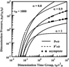 |
Fig. 1 Pressure (unbroken lines) and derivative responses (dashed lines) for subdiffusive flow for α = 0.8. The distance from the well rD is the parameter of interest. The circles and squares correspond to the asymptotic solutions given in equations (22) and (23), respectively. |
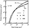 |
Fig. 2 Correlation of well responses indicated in equation (19). Both pressure and derivative responses are considered for values of the distance, rD, in the range 1 ≤ rD ≤ 103. |
 |
Fig. 3 The working Theis solution for subdiffusive flows. |
We now turn our attention to the consideration of the influence of a finite wellbore; see Figure 4 where we consider the influence of rD for α = 0.9. The rD = 1 is the well response for the finite-well-radius case. At long enough times, the pressure response follows the trend suggested in equation (22). Furthermore, at distances rD > 20 the results in Figure 4 suggest that the influence of the well radius will be negligibly small, a conclusion similar to that suggested by Mueller and Witherspoon (1965) for the classical case, α = 1. Figure 5 considers pressure distributions around a well produced through a vertical fracture, equation (26). Results are based on assuming the characteristic length to be the fracture half-length, Lf; rD now given by (31)is assumed to be 1.2. The symbol θ, the parameter of interest, is the orientation of the line on the horizontal plane (y = 0) joining the center of the fracture (xw,yw) to the point r (x−xw,y−yw) with respect to the fracture plane; that is,
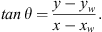 (32)
(32)
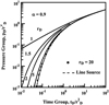 |
Fig. 4 Finite-well-radius solutions obtained by inverting equation (13). The dashed line is the line-source solution, equation (19). At large enough distances (or long enough times) finite-well and line-source responses become indistinguishable. |
 |
Fig. 5 Pressure distribution under subdiffusive flow at rD = 1.2 for a well produced through a vertical fracture; the flux distribution along the fracture length is uniform. The subdiffusive coefficient, α, is 0.8. The compass orientation, θ, in a horizontal plane is the parameter of interest with θ = 0° being aligned with the fracture plane. |
The results shown here are typical of all values of rD except for the fact that the influence of θ diminishes as rD increases and is essentially negligible if rD were greater than 2. This observation, of course, is independent of the subdiffusion coefficient, α. Interestingly, the θ = 90° solution corresponds to the line-source solution, equation (19), if responses are plotted in terms of  vs
vs  . This is one of the reasons why the line-source solution has been often successfully used to evaluate fractured wells. Considering the alignment of the curves, if determining the orientation, θ, is the goal, then choosing a location where θ ≤ 45° should be preferable. At long enough times, behavior similar to that given in equation (23) will be evident for all orientations, θ, and distances, rD. This point may be illustrated by substituting the right-hand side of equation (21) in equation (28) for K0 (z) and integrating with respect to x; see Raghavan and Ozkan (1994). All of these observations in a qualitative sense also apply to situations where the fracture conductivity is finite (Meehan et al., 1989; Mousli et al., 1982).
4 Commentary
Historically, subdiffusive flows in porous rocks have been modeled by considering transient diffusion on a fractal object where the second moment of the distance travelled by the front, <r2>, in terms of the anomalous diffusion coefficient or random walk dimension, dw (>2), is given by (33)
(33)
If dw were equal to 2, then classical diffusion results. Equation (33) is based on the presumption of symmetry and that the diffusivity term, η, in the transient diffusivity equation be of the form (Gefen et al., 1983) (34)where θ > 0 is given by
 (35)
(35)
The stipulation of Gefen et al. (1983) translates to the requirement that both porosity and permeability be dependent on distance, r, namely; see Chang and Yortsos (1990): (36)
(36)
The symbols df, and d in equation (36) represent the fractal (Hausdorff) and Euclidean (d = 1, 2, or 3) dimensions respectively. For 2D problems in subsurface rocks, Beier (1994) recommends that we use df = 2.
In terms of applications to subsurface flow, the requirements of both symmetry and power-law structure specificized in equation (36) impose restrictions if one were to consider issues such as well spacing, fracture spacing (when wells are stimulated by multiple hydraulic fractures), estimation of reserves, location of boundaries, anisotropy, and similar considerations. Beier (1994) recognizes the limitation symmetry imposes on the study of 2D problems as his primary interest was in the application of equation (36) to fractured wells. Nevertheless he proceeds by using equation (36) with the observation that although his solution does “... not strictly carry over to the vertical-fracture geometry” and is thus not valid for all times, his solution is exact during the linear and the pseudoradial flow periods. The analog of Beier’s solution in terms of the Laplace transformation is discussed in Raghavan and Chen (2013a). In addition, to address the matter of symmetry they propose adopting Ball et al. (1987) and using the expression (37)instead of equation (33). Here dwi is the random walk dimension in the direction, i. The analog of the line-source solution corresponding to equation (14) and reflecting equation (37) will now involve
![Mathematical equation: $$ \overline{\Delta p}\left({x}_1,{x}_2\right)\sim f({x}_i,{d}_{\mathrm{wi}},s){K}_{\nu }\left[g({x}_i,{d}_{\mathrm{wi}},s)\right], $$](/articles/ogst/full_html/2019/01/ogst180275/ogst180275-eq70.gif) (38)with ν < 1. Although the structure of the solution may appear different with the appearance of the Kν (x) term, the well response is of the form,
(38)with ν < 1. Although the structure of the solution may appear different with the appearance of the Kν (x) term, the well response is of the form,![Mathematical equation: $$ \Delta p\left({x}_1,{x}_2,t\right)\sim f({x}_i,{d}_{\mathrm{wi}},t){H}_{\mathrm{1,2}}^{\mathrm{2,0}}\left[g({x}_i,{d}_{\mathrm{wi}},t)\right], $$](/articles/ogst/full_html/2019/01/ogst180275/ogst180275-eq71.gif) (39)with the power-law behavior being preserved. This expression, however, still does not address the power-law dependence of permeability and porosity on distance. Our approach addresses this aspect and still preserves the subdiffusive characteristics we desire for a number of problems of interest; see Raghavan and Chen (2013a, b, 2017, 2018), Albinali et al. (2016); it is similar to that used in Benson et al. (2004) in another context.
(39)with the power-law behavior being preserved. This expression, however, still does not address the power-law dependence of permeability and porosity on distance. Our approach addresses this aspect and still preserves the subdiffusive characteristics we desire for a number of problems of interest; see Raghavan and Chen (2013a, b, 2017, 2018), Albinali et al. (2016); it is similar to that used in Benson et al. (2004) in another context.
5 Discussion and concluding remarks
The primary contribution of this work is to provide a “working” solution to evaluate well responses under subdiffusive flow as it is difficult, if not virtually impossible, to address the appearance of the loss of connectivity that is often evident even in environments other than naturally fractured reservoirs; see, for example, derivative responses in Figure 6 taken from Thomas et al. (2005) at a number of wells producing from a variety of geological environments which display near power-law behavior suggesting the existence of spatial scaling of properties. For the responses shown, based on the model discussed here, the slopes of these lines suggest that 0.6 ≤ α ≤ 0.8. The responses are for wells producing distinct fluvial deposits in a number of geographical locations in an exploration context. Consequently, it becomes untenable to tap into fractured-well models if we are circumscribed by the requirement that the classical option be used. We may consider the option that the wells produce commingled deposits where the lateral extent of some of the zones is limited in that these zones deplete during the producing phase and are fed by the more extensive zones during the buildup period (differential depletion, backflow); see Gao et al. (1994). Again, it seems that this option would not be viable in each of these tests when the geological setting does not suggest that this is the case.
 |
Fig. 6 Power-law trends: derivative responses at active wells in fluvial environments. |
Models of the kind discussed here enable us to eschew the option of “simple physics and simple geology” when indeed the responses suggest that the geology is complex. The concept of subdiffusion offers a viable option to evaluate well tests which display near power-law behaviors; as already mentioned, classical methods to address tests of the kind shown in Figure 6 require the conjuring up of counterfactual geological options or ignoring heterogeneity altogether. Models incorporating subdiffusive effects have been shown to be a promising alternative in explaining the performance of shale reservoirs; see Chu et al. (2017, 2018).
Acknowledgments
We thank the referees for their comments. The insights of the editor, Dr. B. Noetinger, significantly improved the contents.
In this Appendix we derive the relevant expressions to determine the well response under subdiffusive flow in the presence of storage and skin effects. The problem is best addressed by Duhamel’s theorem as some subtleties are involved in considering the influence of the skin region under subdiffusive flow.
A.1 Wellbore storage and skin for subdiffusive flow
We first consider matters related to the skin region. Following Hawkins (1956), we find that the effective skin factor,  , is given by the expression
 (40)
(40)
For α = 1, equation (40) reduces to Hawkins’s expression, S, namely, (41)
(41)
In terms of the Laplace transformation, equation (40) corresponds to (42)
(42)
We now proceed as in Agarwal et al. (1970) by considering material balance effects around the wellbore and assuming the skin region to be an infinitesimally thin region around the wellbore with a negligibly small storage capacity. We work in terms of the Laplace transformation. The production rate, q, at the surface is the sum of the wellbore rate, qwb, and sandface rate, qsf; that is, (43)with the wellbore rate given by the expression
 (44)where the symbol C is the storage constant of the well or the unit storage factor, and Δpwf = pi−pwf where pwf is the wellbore pressure. From equation (43) for a constant surface rate, q, we obtain
 (45)where qsfD = qsf/q, and where pwD (t) is the dimensionless wellbore pressure with the dimensionless storage constant, CD, given by
 (46)and
 (47)
(47)
For variable-rate production, q(t), Duhamel’s theorem for the pressure distribution, p(r,t), at any point in time is![Mathematical equation: $$ \frac{2\pi \mathop{k}\limits^\tildeh}{\mu }{\left(\frac{\stackrel{\tilde }{\eta }}{{r}_{\mathrm{w}}^2}\right)}^{\frac{1-\alpha }{\alpha }}\left[{p}_{\mathrm{i}}-p\left(r,t\right)\right]={\int }_0^t q\left(\tau \right){p}_{\mathrm{D}u}^\mathrm{\prime}\left({r}_{\mathrm{D}},t-\tau \right)\mathrm{d}\tau. $$](/articles/ogst/full_html/2019/01/ogst180275/ogst180275-eq81.gif) (48)
(48)
In equation (48),  represents dpDu (rD,t)/dt evaluated at t−τ, and pDu (rD,t) is the appropriate constant-rate (unit-well) solution.
For the situation under consideration, equation (48) yields (49)where
  is the Laplace transform of the unit-well solution, pwDu, and is given by
 (50)and on combining equations (45) and (49), we may show that the well response for the solution that incorporates wellbore storage and skin effects is given by
![Mathematical equation: $$ {\bar{p}}_{\mathrm{wD}}=\frac{{\bar{p}}_{\mathrm{wDu}}}{[1+\mathrm{\Omega }{C}_{\mathrm{D}}{s}^2{\bar{p}}_{\mathrm{wDu}}]}, $$](/articles/ogst/full_html/2019/01/ogst180275/ogst180275-eq86.gif) (51)where pwDu is the CD = 0 solution. Or
(51)where pwDu is the CD = 0 solution. Or![Mathematical equation: $$ {\bar{p}}_{\mathrm{wD}}=\frac{{s}^{2-\alpha }{\bar{p}}_{\mathrm{D}}+{\left(\stackrel{\tilde }{\eta }/{r}_{\mathrm{w}}^2\right)}^{\frac{1-\alpha }{\alpha }}S}{[{s}^{2-\alpha }+{s}^2\mathrm{\Omega }{C}_{\mathrm{D}}({s}^{2-\alpha }{\bar{p}}_{\mathrm{D}}+{\left(\stackrel{\tilde }{\eta }/{r}_{\mathrm{w}}^2\right)}^{\frac{1-\alpha }{\alpha }}S)]}, $$](/articles/ogst/full_html/2019/01/ogst180275/ogst180275-eq87.gif) (52)where pD is the
(52)where pD is the  solution. To account for the influences of storage and skin effects that exist at a flowing well on the pressure responses at an observation well, we may, again, use Duhamel’s theorem; see Chu et al. (1980).
References
- Acuna J.A., Ershaghi I., Yortsos Y.C. (1995) Practical application of fractal pressure-transient analysis in naturally fractured reservoirs, SPE Form. Eval. 10, 3, 173–179. DOI: 10.2118/24705-PA. [CrossRef] [Google Scholar]
- Agarwal R.G., Al-Hussainy R., Ramey H.J. Jr. (1970) An investigation of wellbore storage and skin effect in unsteady liquid flow: I. Analytical treatment, Soc. Pet. Eng. Jour. 10, 3, 279–290. [CrossRef] [Google Scholar]
- Albinali A., Holy R., Sarak H., Ozkan E. (2016) Modeling of 1D anomalous diffusion in fractured nanoporous media, Oil Gas Sci. Technol. - Rev. IFP Energies nouvelles 71, 56. [Google Scholar]
- Arps J.J. (1945) Analysis of decline curves, Trans. AIME 160, 228–247. DOI: 10.2118/945228-G. [CrossRef] [Google Scholar]
- Atangana A., Bildik B. (2013) The use of fractional order derivative to predict the groundwater flow, Math. Probl. Eng. 543026, 9. DOI: 10.1155/2013/543026. [Google Scholar]
- Ball R.C., Havlin S., Weiss G.H. (1987) Non-Gaussian random walks, J. Phys. A: Math. Gen. 20, 12, 4055–4059. DOI: 10.1088/0305-4470/20/12/052. [CrossRef] [MathSciNet] [Google Scholar]
- Beier R.A. (1990) Pressure transient field data showing fractal reservoir structure, Paper 90-04 Presented at the Annual Technical Meeting, Calgary, Alberta, Petroleum Society of Canada. DOI: 10.2118/90-04. [Google Scholar]
- Beier R.A. (1994) Pressure-transient model for a vertically fractured well in a fractal reservoir, SPE Form. Eval. 9, 2, 122–128. DOI: 10.2118/20582-PA. [CrossRef] [Google Scholar]
- Benson D.A., Tadjeran C., Meerschaert M.M., Farnham I., Pohll G. (2004) Radial fractional-order dispersion through fractured rock, Water Resour. Res. 40, W12416. DOI: 10.1029/2004WR003314. [Google Scholar]
- Bodvarsson G.S., Boyle W., Patterson R., Williams D. (1999) Overview of scientific investigations at Yucca Mountain: The potential repository for high-level nuclear waste, J. Contam. Hydrol. 38, 1–3, 3–24. [Google Scholar]
- Camacho-Velázquez R., Fuentes-Cruz G., Vásquez-Cruz M. (2008) Decline-curve analysis of fractured reservoirs with fractal geometry, SPE Reserv. Eval. Eng. 11, 3, 606–619. [CrossRef] [Google Scholar]
- Caputo M. (1967) Linear Models of dissipation whose Q is almost frequency independent-II, Geophys. J. R. Astron. Soc. 13, 5, 529–539. [Google Scholar]
- Carslaw H.S., Jaeger J.C. (1959) Conduction of heat in solids, 2nd edn., Clarendon Press, Oxford, p. 510. [Google Scholar]
- Chang J., Yortsos Y.C. (1990) Pressure-transient analysis of fractal reservoirs, SPE Form. Eval. 5, 1, 31–39. [CrossRef] [Google Scholar]
- Chu W.C., Garcia-Rivera J., Raghavan R. (1980) Analysis of interference test data influenced by wellbore storage and skin at the flowing well, J. Pet. Tech. 32, 1, 171–178. DOI: 10.2118/8029-PA. [CrossRef] [Google Scholar]
- Chu W., Pandya N., Flumerfelt R.W., Chen C. (2017) Rate-Transient analysis based on power-law behavior for Permian wells, Paper SPE-187180-MS, Presented at the SPE Annual Technical Conference and Exhibition, 9–11 October, San Antonio, Texas, USA, Society of Petroleum Engineers. DOI: 10.2118/187180-MS. [Google Scholar]
- Chu W., Scott K., Flumerfelt R.W., Chen C. (2018) A new technique for quantifying pressure interference in fractured horizontal shale wells, Paper SPE-191407-MS, presented at the Annual Technical Conference and Exhibition, 24–28 September, Dallas, TX, USA. [Google Scholar]
- Cinco-Ley H., Meng H.-Z. (1988) Pressure transient analysis of wells with finite conductivity vertical fractures in double porosity reservoirs, Presented at the SPE Annual Technical Conference and Exhibition, 2–5 October, Houston, Texas. DOI: 10.2118/18172-MS. [Google Scholar]
- Cooper H.H., Jacob C.E. (1946) A generalized graphical method for evaluating formation constants and summarizing well-field history, Trans. AGU. 27, 526–534. [CrossRef] [Google Scholar]
- Dassas Y., Duby Y. (1995) Diffusion toward fractal interfaces, potentiostatic, galvanostatic, and linear sweep voltammetric techniques, J. Electrochem. Soc. 142, 12, 4175–4180. [Google Scholar]
- de Swaan-O A. (1976) Analytical solutions for determining naturally fractured reservoir properties by well testing, Soc. Pet. Eng. Jour. 16, 3, 117–122. DOI: 10.2118/5346-PA. [Google Scholar]
- Fetkovich M.J. (1980) Decline curve analysis using type curves, J. Pet. Tech. 32, 6, 1065–1077. [CrossRef] [Google Scholar]
- Flamenco-Lopez F., Camacho-Velázquez R. (2001) Fractal transient pressure behavior of naturally fractured reservoirs, Paper 71591 Presented at the Annual Technical Conference and Exhibition, New Orleans, LA, Society of Petroleum Engineers. DOI: 10.2118/71591-MS. [Google Scholar]
- Gao C., Jones J.R., Raghavan R., Lee W.J. (1994) Responses of commingled systems with mixed inner and outer boundary conditions using derivatives, SPE Form. Eval. 9, 4, 264–271. [Google Scholar]
- Gefen Y., Aharony A., Alexander S. (1983) Anomalous diffusion on percolating clusters, Phys. Rev. Lett. 50, 1, 77–80. DOI: 10.1103/PhysRevLett.50.77. [Google Scholar]
- Hawkins M.F. Jr. (1956) A note on the skin effect, Trans. AIME 207, 356–357. [Google Scholar]
- Henry B.I., Langlands T.A.M., Straka P. (2010) An introduction to fractional diffusion, in: Dewar R.L., Detering F. (eds), Complex physical, biophysical and econophysical systems, World Scientific, Hackensack, NJ, p. 400. [Google Scholar]
- IPCC special report on carbon dioxide capture and storage (2005) Prepared by working group III of the Intergovernmental Panel on Climate Change, in: Metz B., Davidson O., de Coninck H.C., Loos M., Meyer L.A. (eds), Cambridge University Press, Cambridge, United Kingdom and New York, NY, USA, 442 p. [Google Scholar]
- Kim S., Kavvas M.L., Ercan A. (2015) Fractional ensemble average governing equations of transport by time-space nonstationary stochastic fractional advective velocity and fractional dispersion, II: numerical investigation, J. Hydrol. Eng. 20, 2, 04014040. [Google Scholar]
- Le Borgne T., Bour O., de Dreuzy J.R., Davy P., Touchard F. (2004) Equivalent mean flow models for fractured aquifers: Insights from a pumping tests scaling interpretation, Water Resour. Res. 40, W03512. DOI: 10.1029/2003WR002436. [Google Scholar]
- Le Borgne T., Bour O., de Dreuzy J.R., Davy P. (2007) Characterizing flow in natural fracture networks: Comparison of the discrete and continuous descriptions, 437–450, in: Krazny J., Sharp J.M., Groundwater in Fractured Rocks: Selected papers from the Groundwater in Fractured Rocks on Hydrogeology, Prague 2003, Taylor & Francis/Balkema, The Netherlands, 647 pp. [Google Scholar]
- Le Mẽhautẽ A. (1984) Transfer processes in fractal media, J. Stat. Phys. 36, 5–6, 665–676. DOI: 10.1007/BF01012930. [Google Scholar]
- Mainardi M., Pagnini G., Saxena R.K. (2005) Fox H functions in fractional diffusion, J. Comput. Appl. Math. 178, 1–2, 321–331. [Google Scholar]
- Meehan D.N., Horne R.N., Ramey H.J. (1989) Interference testing of finite conductivity hydraulically fractured wells, Presented at the SPE Annual Technical Conference and Exhibition, 8–11 October, San Antonio, Texas, SPE-19784-MS. DOI: 10.2118/19784-MS [Google Scholar]
- Mendes G.A., Lenzi E.K., Mendes R.S., da Silva L.R. (2005) Anisotropic fractional diffusion equation, Physica A: Stat. Mech. Appli. 346, 3–4, 271–283. [CrossRef] [Google Scholar]
- Metzler R., Glockle W.G., Nonnenmacher T.F. (1994) Fractional model equation for anomalous diffusion, Physica A 211, 1, 13–24. [Google Scholar]
- Mousli N.A., Raghavan R., Cinco-Ley H., Samaniego-V F. (1982) The influence of vertical fractures intercepting active and observation wells on interference tests, Soc. Pet. Eng. Jour. 22, 6, 933–944. DOI: 10.2118/9346-PA. [CrossRef] [Google Scholar]
- Mueller T.D., Witherspoon P.A. (1965) Pressure interference effects within reservoirs and aquifers, J. Pet. Tech. 17, 4, 471–474. DOI: 10.2118/1020-PA. [CrossRef] [Google Scholar]
- Nigmatullin R.R. (1984) To the theoretical explanation of the universal response, Phys. Status Solidi B Basic Res. 123, 2, 739–745. [CrossRef] [Google Scholar]
- Nigmatullin R.R. (1986) The realization of the generalized transfer equation in a medium with fractal geometry, Phys. Status Solidi B Basic Res. 133, 1, 425–430. [CrossRef] [Google Scholar]
- Noetinger B., Estebenet T. (2000) Up-scaling of double porosity fractured media using continuous-time random walks methods, Transp. Porous Med. 39, 3, 315–337. [CrossRef] [Google Scholar]
- Noetinger B., Estebenet T., Landereau P. (2001) A direct determination of the transient exchange term of fractured media using a continuous time random walk method, Transp. Porous Med. 44, 3, 539–557. [CrossRef] [Google Scholar]
- Noetinger B., Roubinet D., Russian A., Le Borgne T., Delay F., Dentz M., Gouze P. (2016) Random walk methods for modeling hydrodynamic transport in porous and fractured media from pore to reservoir scale, Transp. Porous Med. 115, 2, 345–385. [CrossRef] [Google Scholar]
- Raghavan R. (2004) A review of applications to constrain pumping test responses to improve on geological description and uncertainty, Rev. Geophys. 42, RG4001. DOI: 10.1029/2003RG000142. [Google Scholar]
- Raghavan R. (2009a) A note on the drawdown, diffusive behavior of fractured rocks, Water Resour. Res. 45, 2, W02502. DOI: 10.1029/2008WR007158. [Google Scholar]
- Raghavan R. (2009b) Complex geology and pressure tests, J. Petrol. Sci. Eng. 69, 181–188. [CrossRef] [Google Scholar]
- Raghavan R. (2011) Fractional derivatives: Application to transient flow, J. Petrol. Sci. Eng. 80, 1, 7–13. DOI: 10.1016/j.petrol.2011.10.003. [CrossRef] [Google Scholar]
- Raghavan R. (2012) Fractional diffusion: Performance of fractured wells, J. Petrol. Sci. Eng. 92–93, 167–173. [CrossRef] [Google Scholar]
- Raghavan R., Chen C. (2013a) Fractured-well performance under anomalous diffusion, SPE Res. Eval. Eng. 16, 3, 237–245, DOI: 10.2118/165584-PA. [CrossRef] [Google Scholar]
- Raghavan R., Chen C. (2013b) Fractional diffusion in rocks produced by horizontal wells with multiple, transverse hydraulic fractures of finite conductivity, J. Petrol. Sci. Eng. 109, 133–143. [CrossRef] [Google Scholar]
- Raghavan R., Chen C. (2017) Addressing the influence of a heterogeneous matrix on well performance in fractured rocks, Transp. Porous Med. 117, 1, 69–102. DOI: 10.1007/s11242-017-0820-5. [CrossRef] [Google Scholar]
- Raghavan R., Chen C. (2018) A conceptual structure to evaluate wells producing fractured rocks of the Permian Basin, Paper SPE-191484-MS, Presented at the Annual Technical Conference and Exhibition, 24–28 September, Dallas, TX, USA. [Google Scholar]
- Raghavan R., Ozkan E. (1994) A method for computing unsteady flows in porous media, Pitman Research Notes in Mathematics Series (318), Longman Scientific & Technical, Harlow, UK, 188 p. [Google Scholar]
- Romeu R.K., Noetinger B. (1995) Calculation of internodal transmissibilities in finite-difference models of flow in heterogeneous media, Water Resour. Res. 26, 2, 291–306. [Google Scholar]
- Sanchez-Vila X., Guadagnini A., Carrera J. (2006) Representative hydraulic conductivities in saturated groundwater flow, Rev. Geophys. 44, RG3002. DOI: 10.1029/2005RG000169. [Google Scholar]
- Saxena R.K., Mathai A.M., Haubold H.J. (2006) Fractional reaction-diffusion equations, Astrophys. Space Sci. 305, 3, 289–296. [Google Scholar]
- Schad H., Teutsch G. (1994) Effects of the investigation scale on pumping test results in heterogeneous porous aquifers, J. Hydrology 159, 61–77. [CrossRef] [Google Scholar]
- Stehfest H. (1970a) Algorithm 368: Numerical inversion of Laplace transforms [D5], Commun. ACM 13, 1, 47–49. [Google Scholar]
- Stehfest H. (1970b) Remark on algorithm 368: Numerical inversion of Laplace transforms, Commun. ACM 13, 10, 624. [Google Scholar]
- Su N., Nelson P.N., Connor S. (2015) The distributed-order fractional diffusion-wave equation of groundwater flow: Theory and application to pumping and slug tests, J. Hydrology 529, 1262–1273. [Google Scholar]
- Theis C.V. (1935) The relationship between the lowering of the piezometric surface and the rate and duration of discharge of a well using ground-water storage, EOS Trans. AGU 2, 519–524. [Google Scholar]
- Thomas O.O., Raghavan R., Dixon T.N. (2005) Effect of scaleup and aggregation on the use of well tests to identify geological properties, SPE Res. Eval. Eng. 8, 3, 248–254. DOI: 10.2118/77452-PA. [CrossRef] [Google Scholar]
- Uraiet A., Raghavan R., Thomas G.W. (1977) Determination of the orientation of a vertical fracture by interference tests, J. Pet. Tech. 29, 1, 73–80. DOI: 10.2118/5845-PA. [CrossRef] [Google Scholar]
- Warren J.E., Price H.S. (1961) Flow in heterogeneous media, Soc. Pet. Eng. Jour. 1, 3, 153–169. [CrossRef] [Google Scholar]
- Warren J.E., Root P.J. (1963) The behavior of naturally fractured reservoirs, Soc. Pet. Eng. Jour. 3, 3, 245–255. DOI: 10.2118/426-PA. [Google Scholar]
- Weisstein, E.W. (2018) Fox H-Function. From MathWorld – A Wolfram web resource. http://mathworld.wolfram.com/FoxH-Function.html; see also, http://www.wolframalpha.com/input/?i=fox+h-function. [Google Scholar]
- Whiting R.L., Ramey H.J. (1969) Application of material and energy Balances to geothermal steam production, J. Pet. Tech. 21, 7, 893–900. DOI: 10.2118/1949-PA. [CrossRef] [Google Scholar]
All Figures
|
Fig. 1 Pressure (unbroken lines) and derivative responses (dashed lines) for subdiffusive flow for α = 0.8. The distance from the well rD is the parameter of interest. The circles and squares correspond to the asymptotic solutions given in equations (22) and (23), respectively. |
| In the text | |
|
Fig. 2 Correlation of well responses indicated in equation (19). Both pressure and derivative responses are considered for values of the distance, rD, in the range 1 ≤ rD ≤ 103. |
| In the text | |
|
Fig. 3 The working Theis solution for subdiffusive flows. |
| In the text | |
|
Fig. 4 Finite-well-radius solutions obtained by inverting equation (13). The dashed line is the line-source solution, equation (19). At large enough distances (or long enough times) finite-well and line-source responses become indistinguishable. |
| In the text | |
|
Fig. 5 Pressure distribution under subdiffusive flow at rD = 1.2 for a well produced through a vertical fracture; the flux distribution along the fracture length is uniform. The subdiffusive coefficient, α, is 0.8. The compass orientation, θ, in a horizontal plane is the parameter of interest with θ = 0° being aligned with the fracture plane. |
| In the text | |
|
Fig. 6 Power-law trends: derivative responses at active wells in fluvial environments. |
| In the text | |