Regular Article
Towards an integrated restoration/forward geomechanical modelling workflow for basin evolution prediction
1
Three Cliffs Geomechanical Analysis Ltd,
Swansea,
Wales, UK
2
Swansea University,
Swansea, UK
3
Chevron Energy Technology Company,
1500 Louisiana St,
Houston,
TX
77002, USA
* Corresponding author: e-mail: This email address is being protected from spambots. You need JavaScript enabled to view it.
Received:
2
February
2018
Accepted:
25
April
2018
Abstract
Many sedimentary basins host important reserves of exploitable energy resources. Understanding of the present-day state of stresses, porosity, overpressure and geometric configuration is essential in order to minimize production costs and enhance safety in operations. The data that can be measured from the field is, however, limited and at a non-optimal resolution. Structural restoration (inverse modelling of past deformation) is often used to validate structural interpretations from seismic data. In addition, it provides the undeformed state of the basin, which is a pre-requisite to understanding fluid migration or to perform forward simulations. Here, we present a workflow that integrates geomechanical-based structural restoration and forward geomechanical modelling in a finite element framework. The geometry and the boundary kinematics derived from restoration are used to automatically create a forward geomechanical model. Iterative correction may then be performed by either modifying the assumptions of the restoration or modifying the restoration-derived boundary conditions in the forward model. The methodology is applied to two problems; firstly, a sand-box scale benchmark model consisting of sand sediments sliding on silicon leading to the formation of a graben structure; secondly, a field-scale thrust-related anticline from Niger Delta. Two strategies to provide further constraint on fault development in the restoration-derived forward simulation are also presented. It is shown that the workflow reproduces the first order structural features observed in the target geometry. Furthermore, it is demonstrated that the iterative approach provides improved understanding of the evolution and additional information of current-day stress and material state for the Niger Delta Case.
© A.J.L. Crook et al., published by IFP Energies nouvelles, 2018
 This is an Open Access article distributed under the terms of the Creative Commons Attribution License (http://creativecommons.org/licenses/by/4.0), which permits unrestricted use, distribution, and reproduction in any medium, provided the original work is properly cited.
1 Introduction
Sedimentary basins are complex natural systems, which are a few to several hundred million years old and which constitute the human exploitable source for fossil energy and some of the geothermal energy resources. The information and data concerning structural configuration, sediment properties and fluid composition that can be measured (mostly indirectly and with limited resolution/spatial extent) from sedimentary basins is just a snapshot of the present-day state. These parameters and properties have, however, evolved with time since early stages of basin formation to the present-day via a combination of numerous processes such as sediment deposition, subsidence and burial, sediment compaction, diagenesis, sediment lithification, fluid over pressure development, fluid and heat flow, oil generation and migration, fault initiation and offset, deformation due to tectonic activity, etc. Thus, understanding such complex evolution is crucial in order to minimize uncertainty in basin state at present day and optimize resource exploitation.
Basin modelling is a tool used to predict vertical stress, pore pressure, temperature, porosity, fluid flow and oil migration histories, thereby decreasing uncertainty in the present-day basin status (e.g. Schneider et al., 1996; Hantschel and kauerauf, 2009; Faille et al., 2014; Estublier et al., 2017). The technique often relies on porosity – “vertical effective stress” or porosity – “effective mean stress” relationships to represent compaction (e.g. Bolås et al., 2004; Gutierrez and Wangen, 2005), and therefore only approximately accounts for the geomechanical evolution. Additionally the influence of faults on both the strain field and fluid flow (Woillez et al., 2017) are also approximate. This may lead for example to poor stress prediction in faulted zones, poor modelling of fault behaviour (Thibaut et al., 2014) and underestimation of compaction and/or of pore pressure generation in tectonic dominated basins (Obradors-Prats et al., 2017b).
On the other hand forward geomechanical basin modelling simulates evolutionary basins by solving the governing equations and incorporating sophisticated constitutive models that capture the physics underlying the system. This methodology has been widely employed by earth scientists to investigate the influence of different geological parameters in basin evolution and make predictions of present day basin geometries, stresses and pore pressure distribution (e.g., Kjeldstad et al., 2003; Peric and Crook, 2004; Bernaud et al., 2006; Crook et al., 2006; Albertz and Lingrey, 2012; Albertz and Sanz, 2012; Luo et al., 2012; Nikolinakou et al., 2012; Smart et al., 2012; Maghous et al., 2014; Nikolinakou et al., 2014; Thornton and Crook, 2014; Roberts et al., 2015; Obradors-Prats et al., 2016; Luo et al., 2017; Obradors-Prats et al., 2017a; Ruh, 2017).
The main ingredients required to develop a forward geomechanical model are; (a) the initial paleo-geometry, (b) the constitutive relationships for all the sediments within the model domain and, (c) the evolving boundary conditions. When the goal is to predict and match a structure observed, either from the field or from a sandbox experiment, a proper definition of these ingredients is essential.
Structural restoration (also known as reverse modelling) is a technique to ‘undeform’ a present-day geometry back to its original state or to a target paleo time. Structural restoration is applied to both validate structural interpretations made from seismic data and to infer past deformation states of geological structures, shedding light on the basin history and the kinematics involved in basin evolution (e.g. Dahlstrom, 1969; Boyer and Elliott, 1982; Gibbs, 1983; Kusznir et al., 1995; Maerten and Maerten, 2006; Guzofski et al., 2009; Durand-Riard et al., 2011; Durand-Riard et al., 2012; Lovely et al., 2012; Rowan and Ratliff 2012; Durand-Riard et al., 2013; Lopez-Mir et al., 2014; Nyantakyi et al., 2014) A structural restoration can, therefore, provide the initial paleo-geometry and evolving boundary conditions for geomechanical forward models.
Here, we present a workflow that integrates geomechanical based restorations and forward geomechanical modelling within the same finite element code (ParaGeo). The integrated framework facilitates direct transfer of the restoration derived geometry and kinematics to the forward model definition. In addition, we discuss how this framework can be employed to perform corrections into restoration assumptions based on the restoration-derived forward simulation results. Correction may be performed, either after a complete cycle of restoration and forward simulation (incremental scheme), or after restoration and forward simulation at each restoration step (iterative correction). By employing the corrective schemes both, restoration and forward simulation are enhanced simultaneously.
We demonstrate the methodology by application to a synthetic sandbox scale extensional benchmark model consisting of sand-like sediments gravitationally sliding on a silicon base layer. In addition, we discuss and illustrate two different techniques that can be employed to activate faults within forward models in order to provide further constraint to geometry evolution. We first demonstrate the usage of “fault seeding”, where localised weakening of material strength facilitates a localisation, which is indicative of brittle faulting, using the sandbox extensional benchmark and we show the influence of fault seeding on the predicted geometry. Secondly, we demonstrate a fault insertion algorithm, which inserts and extends discrete faults, represented using contact surfaces, into newly deposited formations using a field-scale thrust-related fold structure from Niger Delta. The field scale Niger Delta example also demonstrates that iteration on the incremental approach provides improved understanding of the evolution and the current-day strain (porosity) distribution.
2 Restoration methodology
Restoration of geological structures (also known as inverse modelling) consists of performing a retro-deformation sequence of the target structure to a target paleo time in order to; (a) infer the evolution of the paleo-geometry, and (b) validate structural interpretations developed from seismic data.
Classical or kinematic structural restoration is based on purely geometrical procedures that consist in back stripping the top surface horizon to an assumed restoration surface using geometric and kinematic constraints. In other words, the deformed top stratigraphic surface is “unfolded” to its assumed initial, undeformed configuration, and this process is repeated for each stratigraphy unit sequentially by deactivating the top unit after each restoration step. It should be noted that the restoration of a particular geological structure can be performed assuming different kinematic scenarios and to this end many different constraints have been proposed; e.g. cross section area and line-length balancing (e.g. Gibbs, 1983; Rowan and Kligfield, 1989), bedding-plane slip (e.g. Griffiths et al., 2002), vertical or inclined shear (e.g. White et al., 1986), tri-shear (e.g. Hardy and Finch, 2007; Spinelli et al., 2007) and quad-shear (e.g. Welch et al., 2009).
Finite Element (FE) based restoration has been proposed as an alternative to the classical approach (e.g. Muron, 2005; Maerten and Maerten, 2006; Moretti et al., 2006; Guzofski et al., 2009; Durand-Riard et al., 2011; Durand-Riard et al., 2013; Chauvin et al., 2018). Using this approach the basic concept of back stripping the top surface to a restoration surface is maintained but a FE model is used where sediment blocks interact via contact surfaces representing the faults. A vertical displacement is imposed to the model top surface nodes so that at the end of the restoration step it coincides with the imposed restoration surface, whereas the horizontal component of the displacement is usually free, allowing for extension/compression of the model (Fig. 1). A key difference with classical restoration approaches is the deformational behaviour of the sediments. Area and volume conservation (which are proxies for mass conservation) are not imposed directly but rather the sediments within the structure behave according to an elastic constitutive relationship honouring mass conservation. Both linear isotropic and transverse isotropic models have been proposed, with the latter having some benefit when bedding-plane slip is important (e.g. Durand-Riard et al., 2012). But more advanced modelling of bedding plane slip, either by a distributed planes-of-weakness (e.g. Fujii, 2012; Fujii et al., 2013) type model, or discrete contact surfaces can also be introduced (Fig. 2). Line length preservation of the top surface can optionally be imposed by introduction of additional constraint equations. Faults are defined by means of frictionless contact surfaces with an imposed normal stiffness to minimize mesh penetration between adjacent fault blocks. The frictionless condition minimises shear tractions adjacent to the sliding surfaces ensuring that undesired deformation features produced by the reverse motion do not arise.
Depositional-based problems are addressed by the incorporation of a decompaction law. The model is first initialized with a porosity distribution established from current-day observations. Then decompaction is performed during each step of the restoration according to a prescribed compaction trend with depth. The compaction trend may vary as a function of time; e.g. due to changes in overpressure distribution or diagenesis. Decompaction may be performed sequentially after each restoration step or as in the case for ParaGeo it may be active over the complete restoration step so that the increase in sediment thickness is smoothly changing as a function of time.
Clearly, the simplistic assumptions of both restoration techniques cannot fully represent the true physical evolution, and combining these techniques with a more sophisticated geomechanical forward model offers clear potential for improving the quality of predicted evolution.
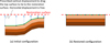 |
Fig. 1 Schematic example of the boundary conditions adopted for back striping the top surface to a restoration surface. (a) Initial geometry configuration (present day), (b) restored geometry configuration. |
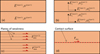 |
Fig. 2 Schematic representation of several restoration options available in ParaGeo. (a) Isotropic elasticity, (b) transverse isotropic elasticity, (c) distributed intra-layer bedding plane slip model and (d) inter-layer bedding plane slip using contact surfaces. |
3 Forward simulation methodology
3.1 Governing equations
The computational framework incorporates finite strain and adaptive remeshing procedures (Peric and Crook, 2004) and adopts a Lagrangian methodology that incorporates:
-
large deformations of inelastic solids at finite strains;
-
constitutive modelling of generic inelastic material suitable for description of plastic, viscoplastic and viscoelastic behaviors that may be active simultaneously;
-
an adaptive strategy for modelling of large deformations of inelastic solids at finite strains;
-
energy regularization based on extension of the fracture energy concept.
The geomechanical field adopts linear momentum balance equation for a saturated medium containing a single fluid phase as described in Lewis and Schrefler (1998). This formulation adopts Biot theory to define the total stress as a function of the effective stress and pore pressure and a nonlinear Biot coefficient dependent on porosity.
For the applications described in this work, hydrostatic pore pressures are assumed. The flow field is not solved and pf is rather evaluated based on fluid density and current depth (water height) at each mechanical step. Temperature field is neither solved or prescribed as, for the sake of simplicity, the simulations presented neglect all temperature dependent processes.
3.2 Constitutive model
The constitutive model must account for both mechanical and non-mechanical evolution. For example, chemical diagenesis may induce an overprint in sediment geomechanical properties such as porosity and strength (e.g. Nygård et al., 2004a, b; Nygård et al., 2006) that strongly influences the deformational response and fluid migration pathways.
Mechanical compaction is represented using a critical state constitutive model named SR4 (e.g. Obradors-Prats et al., 2016; Obradors-Prats et al., 2017a, b). This is a variation of the modified Cam Clay Model (Wood, 1990) with added flexibility in the definition of the yield surface shape and a non-associative flow rule. In critical state theory the critical state line divides the yield surface in two regions; the cap side and the shear side. When stress paths intersect the yield surface on the cap side (to the right of the critical state line) compaction occurs, the yield surface increases in size so that the material hardens (increase in strength). Conversely when stress paths intersect the yield surface on the shear side (to the left of the critical state line) dilation occurs, the yield surface decreases in size so that the material softens (decrease in strength). When stress paths intersect the yield surface at critical state continuous shear occur without any change in volume nor stress state.
Non-mechanical compaction is used here to define all time dependent process that are not represented in the standard geomechanical constitutive model; e.g. diagenesis, creep, sub-critical fracture propagation, etc. These processes are dependent on the microstructure of the formation, fluid constitution, temperature and time, and include: early carbonate cementation, Opal A/CT (>25°) Transition, Smectite-Illite (>65°) Transition and Kaolinite to Illite (>120°) Transition. The influence of these processes on the mechanical properties is represented by defining a set of generic reaction laws dependent upon constitutive properties and the temporal variation of temperature such that each reaction characterises (Crook, 2013):
-
a specific maximum porosity change;
-
a tensile strength increase; due to cementation;
-
a compressive strength increase; due to change in the microstructure;
-
the change in Cam Clay material parameters, λ and k, which govern compaction and unloading respectively.
3.3 Adaptive remeshing algorithm
Large strain problems require remeshing operations to be performed routinely during the simulation in order to prevent excessive mesh distortion and also to provide a spatial distribution of mesh density that captures high-gradient deformation features such as faults while we keep relatively coarse non-active zones of the model domain. After remeshing, both the primary and history-dependent state variables are transferred from the old mesh to a new mesh using a procedure outlined in Peric and Crook (2004).
4 Iterative restoration/forward modelling methodology
4.1 Methodology
Forward geomechanical modelling requires definition of both the initial geometry configuration and the temporal variation of the boundary conditions, i.e. the boundary evolution, sedimentation/erosion history, and fluid/heat flux across the boundary. Some of this data can be derived from restoration results. As mentioned in Section 2, however, the simplistic assumptions in restorations only loosely represent the processes occurring in nature. Consequently, a new class of inverse modelling techniques that enable rational combination of restoration and forward modelling needs to be established. This workflow couples geological restoration analysis with predictive, geometrically unconstrained or partially constrained, geomechanical forward modelling analysis. Solution convergence is based on the objective of reproducing the current-day geometry. An additional benefit of this approach is that, unlike standard restoration, the full history of stress, pore pressure, fluid migration and material state are predicted by the forward model.
Coupling restoration and forward analysis can be achieved by employing either an incremental (restoration assumptions are modified after complete restoration) or an iterative (restoration assumptions are modified after each restoration step) approach (Fig. 3). In either case the solution derived from the restoration is used to drive the forward model to the current-day and the consistency between the predicted and observed geometry is used to evaluate whether corrective steps should be performed. These may be applied via either modification of the restoration assumptions (e.g., apply additional extension due to a mismatch in the lateral compaction) or the boundary conditions of the forward model (e.g. direct modification of the boundary displacements). It should be noted that such modifications are currently applied manually after analysing and assessing the results but the process may be automated by introducing some constrains and numerical optimization techniques.
It should be noted that, although FE-based restoration models are adopted here, coupling of restoration and forward modelling is also applicable to classical restoration techniques.
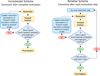 |
Fig. 3 Flowcharts for improving restorations following an integrated workflow of restoration and forward simulation. |
4.2 Restoration → forward model construction
The forward simulation model is constructed automatically using the restored geometry. This is achieved by processing the restored geometry at the end of each restoration step and the tracking of the displacements of the model boundaries over the restoration step. Boundary displacements are evaluated by linear interpolation between the initial and final positions of each node on the model boundary. This defines both, the boundary displacement and, in conjunction with the restoration surface, the geometry (isopach) of the layers to be deposited during forward simulation.
The discretisation of the restoration and forward models may be fundamentally different as faults in the restoration are always represented as discrete, frictionless contact surfaces, whereas in the forward model they may be either; (a) not defined, (b) seeded within a continuum mesh, or (c) defined by a discrete, contact surface with friction. For cases (a) and (b) the restoration model output must therefore be “stitched” across the fault when deriving the forward model. Additionally, the evolution of the forward model will always diverge to some extent from the restoration. Consequently, even if a fault is represented as discrete in the restoration and the forward model, the precise location of the fault may differ when the fault is propagated to a new sedimented layer.
To facilitate consistency between disparate discretisations, the geometry of the restored basal and side boundaries is converted to “part geometry” entities; i.e. geometry lines, points and surfaces that are independent of the model mesh and domain. These part geometries drive the motion during the forward model simulation by applying the tracked restoration displacement in a reverse sense. The relationship between the model boundary and the part boundary is dependent on the boundary type. A “tied” condition (no relative displacement) is generally imposed on the basal horizon lines enforcing the model mesh to deform consistently with the basement part geometry. This ensures full consistency between restoration and forward model boundary displacements and facilitates the prediction of deformational structures at precise locations observed in the target geometry. Faults on the basal boundary are either represented using prescribed displacement, via a specialized fault boundary where the fault elongation is assumed to occur locally in the top segment edge (the fault tip), or via a frictional slip condition imposed via a general contact algorithm. For lateral boundaries, a frictionless contact condition is imposed so that the displacements are only prescribed perpendicular to the part geometry entities. This is beneficial as it facilitates compaction due to deposition and/or thickening due to shortening with minimization of potential boundary effects (i.e. if friction or fully prescribed displacements condition are applied to lateral boundaries shear deformational features may arise nearby).
During the forward simulation the displacements relative to the subsidence are applied before the sedimentation of a layer. This ensures that the accommodation space needed for its deposition is achieved prior to sedimentation. The sediments are deposited either with an uncompacted or a pre-compacted state, with porosities that follow a prescribed compaction trend, consistent with the decompaction porosity trend to ensure deposition of the correct mass of solids.
4.3 Illustrative example
4.3.1 Procedure
A 2D plane strain forward model that represents gravitational sliding of brittle sediment on a ductile base-layer is used to generate a “target” present-day geometry. The advantage of using a target geometry derived from a forward model to validate the methodology is that the constitutive models are well constrained and the complete displacement and strain history are known. In addition, the restoration surface is also known (which in field cases has to be assumed) as it is defined according to the deposition horizon. This target geometry is restored, using isotropic elastic assumptions, and then a forward model is generated, simulated and compared with the original Target model. The configuration and results for the Target model are described in Appendix 1 and material parameters are listed in Appendix 2 (Table A1 and Table A2).
4.3.2 Restoration model description
The restoration model comprises elastic fault blocks separated by contact surfaces, created by interpretation of the Target model geometry in final configuration (see the top plot of Fig. 4). All major faults and 4 secondary faults are explicitly discretized. Faults are defined with a frictionless contact condition so that fault blocks can freely slide on each other. The restoration surface is tilted with a slope identical to the slope of the sedimentation horizon used to generate the target geometry (see Fig. A1).
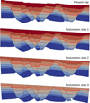 |
Fig. 4 Restoration sequence from present day to restoration step 3. The red curve indicates the tracked geometry horizon that will define the boundary conditions for the forward simulation. |
4.3.3 Restoration results and forward simulation description
The three restoration steps capture the flattening of the top horizons of the three youngest formations (Fig. 4). Restoration recovers part of the total fault offset for most faults measured at the red horizon in Figure 4, with full recovery for the fault second from the left of the model. The basal shape of the third youngest formation is tracked so that it can be later applied as a boundary condition for the forward simulation with a fully fixed condition on the horizon lines and frictional sliding on the fault lines adjacent to the boundary. The shape and position of the lateral boundaries are also tracked and applied as frictionless boundary in the forward simulation. The sedimentation horizon for the forward simulation is defined from the restoration datum surface (Fig. 5).
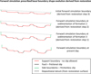 |
Fig. 5 Forward simulation prescribed basal boundary shape evolution derived from restoration. |
4.3.4 Forward model results and comparison to Target model results
The results of the target and the predicted models are compared via the predicted geometry and plastic strain contour distribution (Fig. 6). The restoration-derived forward simulation captures the first-order structural features of the target simulation, especially the features related to faults with large offset. Conversely faults with low offset are more poorly represented, particularly the step-like surface expression related to faults projected to the top surface. The predicted fault angles compare favourably with those of the Target model with slight differences. For the faults that can be clearly measured in the plastic strain contour plots the average difference in fault angle is 3.6° with a maximum difference of 10.7° measured on the second synthetic fault starting to the left and a minimum difference of 0.0° measured on several faults. The offset for both simulations is similar but it differs locally in some regions. For example, the synthetic fault framed by the red rectangle (Fig. 6) shows larger offset in the Target model, possibly due to differences in the internal displacement distribution (e.g. note that strain localization in the restoration-derived forward simulation branches into two thin localization paths in the two top formations, thus accommodating the offset in a wider zone whereas in the target simulation only a single fault accommodating the total offset is visible).
The differences observed between the Target model and the restoration-derived forward simulation could be explained by several reasons. Firstly, the results are dependent on the restoration model structural discretization, interpreted from the Target model. As the Target model is continuum, faults are represented by strain localization in a finite width which, in our simulations, are of the order of 1 mm (i.e. 4–5 of the smallest elements). These are represented by discrete faults with zero width in the restoration model. This results in an approximate representation that has sharper changes in basal boundary geometry (e.g. compare the shape of the base in Figs. 6a and b). This modifies the prescribed boundary displacement which in turn can lead to perturbations in the internal distribution of strain and therefore in predicted structural features. Similarly, the different constitutive model assumptions in the forward geomechanical and restoration simulations (i.e. elasto-plastic vs. elastic) will also influence the solution. For example, large distributed shear strains cannot be recovered during restoration and horizon/fault intersection geometry is generally more abrupt than in the Target model. Another potential issue is the linear interpolation of the model boundary movement over each restoration step. If fault block rotation occurs within a given step, the transferred displacements to the forward simulation might be an oversimplification of the true kinematics. Fault block rotation is common in viscoelastic-driven tectonic scenarios such as this example. It should be noted as well that the total net horizontal extension measured in the benchmark model has not been fully recovered during restoration because restoration cannot recover the extension produced by continuum deformation or faults that have not been considered during discretization. Consequently the restoration-derived forward simulation predicts less horizontal extension (26.9 cm) than the benchmark model (39.5 cm).
It should be reinforced that the most of the differences are, however, second order and that the coupling of restoration and forward simulation is successful in reproducing the main structural features. In addition, it should be noted that iterative correction of neither the restoration discretization nor the forward model has been performed in this case.
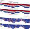 |
Fig. 6 Comparison of final configuration geometries and plastic strain contours for the Target model (a) and (c) and the restoration-derived forward simulation (b) and (d). |
5 Fault seeding and fault insertion
In some circumstances, a forward analysis using restoration-derived boundary conditions may predict results that diverge from the target geometry. This may be indicative of either; (a) incompatible assumptions in the restoration or the forward model (e.g. the reversal of the displacements derived from the restoration are not fully representative of the displacements that drove the evolution of the target structure), or (b) a scenario where small variation in the conditions (e.g. in the stress field distribution) result in a different structure evolution (e.g. formation of antithetic or synthetic faults). In addition, for basin-scale problems the time-history of evolution of the state boundary surface can only be inferred from current-day observations, but its form, together with the material characterisation, controls the transition from ductile to brittle behaviour in sediments. Consequently, given that the restoration derived boundary conditions are also imprecise, a fully-free forward simulation may diverge significantly from the target geometry; e.g. prediction of an antithetic rather than a synthetic fault early in the solution may completely change the final structure. It is, therefore, often desirable to condition the forward model to predict a present-day geometry that is representative of the target geometry by providing further constraint to the structure evolution.
Fault-triggering strategies; i.e. definition of the model locations and orientations where faults are expected to develop, fall into this category. Fault-triggering may be achieved by; (1) tracking the shape and architecture of faults during the restoration, (2) transferring the fault geometry, as geometry independent of the mesh to the forward model and (3) triggering or extending faults in the forward model using the restoration fault geometry. At each sedimentation step, some or all interpreted faults are propagated into the newly sedimented layer via either (see Fig. 7):
-
Fault seeding; i.e. decreasing the strength for the elements which are on the fault trace to increase the probability of fault propagation via strain localization along the fault trace. This constitutes a weak constraint as fault propagation is not explicitly enforced.
-
Fault insertion; i.e. splitting the model along the fault trace and inserting a discrete fault with a frictional contact condition. This constitutes a strong constraint on structure evolution.
It is important to note, however, that both methods of fault-triggering are a “nudge” rather than an absolute constraint, so that if either the boundary conditions derived from the restoration or the material characterisation are inappropriate this will still be evident in the forward model predictions. Fault seeding or insertion can also be applied selectively; e.g. to major faults, facilitating gross deformation patterns consistent with current-day observations, but providing free evolution in regions of particular interest.
The seeding and fault insertion methodologies have different demands in terms of mesh generation. Fault seeding requires a fine mesh along the fault trace to provide sufficient kinematic freedom to properly propagate a strain localization of thin finite width, otherwise the displacement gradients may not be representative of faulting. On the other hand, as fault insertion splits the mesh providing a discrete contact surface, the mesh can be much coarser with the drawback that mesh generation becomes more difficult as complexity in geometry increases (note that the more the geometry is split, the more constrains imposed to the mesh as it should conform to all geometry lines).
An example of fault seeding is shown in Figure 8. This model corresponds to the target simulation described in Appendix 1: Benchmark model, with the exception that three right-dipping faults, with a slope of 60°, are seeded. Seeding is via a positive (0.05) volumetric strain, locally reducing the pre-consolidation pressure (strength decrease) along the fault path. Consequently, initial brittle faulting of the sand layer via localised deformation is more likely to be preferentially accommodated in these weaker zones rather than the surrounding intact material. Subsequently the model is not prescribed with any further fault seeding.
The influence of prescribing fault seeding within the pre-kinematic sand layer is evident in structure evolution (Fig. 9). The seeded synthetic faults are close to optimal in terms of location and dip and consequently subsequent deformation is primarily accommodated by offset and sliding (high plastic strain) on these faults. The maximum offset is observed in the second fault; 31 mm measured at the pre-kinematic sand top horizon. The average fault angles range from 47.4° to 60.6°. Antithetic faults are much less developed than in the fully-unconstrained simulation (compare Fig. 9 and Fig. A3).
The key point is that the location and form of the initial brittle failure of the sand layer is not strongly constrained by the geometry and is sensitive to any imperfections in the properties of the sand layer. This is true for both, sand-box experiments and the model. Consequently, seeding pre-defined imperfections, which can be quite small, can condition a model to evolve towards a target geometry without strongly enforcing this constraint.
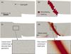 |
Fig. 7 Examples of the two fault triggering methods, fault insertion (a), (c) and fault seeding (b) and (d). Figures (a) and (b) show undeformed geometries with the initial conditions at fault location. Note that the fault path in (a) is used to split the continuous geometry at early stages of the simulation. Figures (c) and (d) show the model mesh after the first deformational stage of the simulation. |
 |
Fig. 8 Schematic model initial geometry showing the location of the seeded faults. |
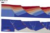 |
Fig. 9 Predicted geometry (a) and plastic strain contours (b) at the upper edge of the model after deposition of five layers for the case with fault seeding. |
6 Field-scale coupled restoration/forward model
6.1 Overview
The combined restoration/forward modelling methodology is applied to a field scale structure, including compaction, and demonstrates the benefit of using the fault insertion algorithm relative to a freer algorithm where faults are not seeded or inserted, so can only arise naturally via continuum strain localisation.
The current-day geometry comprises a thrust-related anticline in the Niger Delta (Higgins et al., 2009). It is approximately 6.5 km wide, measured from the two points where the horizon h8 in the backlimb and forelimb respectively exhibit initial curvature, and deviates from the sub-horizontal direction with maximum amplitude of 607 m (Fig. 10a). The backlimb is notably longer than the forelimb and has a lower average dip (11.0°) compared to the forelimb (23.1°). The thrust fault is approximately 3.3 km long and dies out within formation 9 (bounded by horizon h9 at top and horizon h8 at the base (see horizon numbers in Fig. 10a). It has an average slope of 50.4° and is non-uniformly curved, changing from a concave shape at the deep section to a convex shape in its shallowest part. The maximum slip for the thrust is 620 m measured at horizon h3. A near straight backthrust, with a slope of 33.9°, cuts horizon h2 and horizon h3 and accommodates a relatively small offset of 30 m.
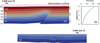 |
Fig. 10 (a) Restoration model for an isolated thrust structure from Niger Delta. The geometry has been obtained from Higgins et al. (2009). The horizons are numbered consistently with the reference; i.e. h1 for the model base to h11 for the top surface. Note that intra-formation fault tips have been neglected. (b) Prescribed initial porosity distribution with depth. This porosity distribution is representative of Niger Delta sediments and has been obtained from the field data published by Krueger and Grant (2011). (c) Final restored geometry after restoration of 8 formations. |
6.2 Restoration
The deepest formation which contains the detachment is omitted from the restoration so that the boundary displacements from the restoration directly apply offset on the thrust in the forward simulation. The model is pinned at the right-hand boundary (zero horizontal displacement) and a flat, horizontal restoration surface is prescribed slightly above the current-day top surface (Fig. 10a). The remaining boundaries are free. Frictionless contact surfaces are defined on faults. During restoration, vertical decompaction is performed using the vertical effective stress − porosity relationship for Niger Delta sediments described in Figure 10b from Krueger and Grant (2011), and assuming hydrostatic pore pressure (Fig. 10b). The initial porosity distribution throughout the model is also prescribed using this trend. Eight restoration steps are performed until horizon h4 is flattened, which according to Higgins et al. (2009) is the top of the pre-kinematic section of sediments. The resulting restored geometry which will serve as the initial geometry for the forward simulation is shown in Figure 10c.
6.3 Forward model
The restoration geometry and displacement history of the base and lateral boundaries define both initial forward model geometry and the evolving boundary conditions for the forward simulation. The layers are deposited with a pre-compacted porosity distribution using a porosity trend (Fig. 10b) ensuring that the mass of solids deposited is consistent with restoration and the target field data. Additionally, the hardening properties for the constitutive model are also derived from this porosity trend. The input material properties are summarized in Table A1.
Unlike the simple extensional sandbox case, where the sediment internal to the fault blocks are essentially undeformed, the sediment adjacent to the fault and in the anticline are subjected to significant strain in the present-day configuration. This is not fully captured by the restoration if only vertical decompaction is considered and lateral strains are not recovered. Consequently, the restored bed length and boundary displacements are underestimated by the restoration and this is evident in the forward model predictions which exhibit too little fault offset (see Fig. 11b). Either the restoration or the boundary conditions in the forward model must, therefore, be iteratively corrected until a reasonable match is achieved between the predicted and current-day geometries. In this case additional shortening is introduced to the forward model boundary conditions following the incremental approach shown in Figure 3 until the predicted fault offset matches the observation.
Two simulations are shown; one in which we propagate the faults by fault insertion each time a new formation is sedimented as described in section 5 and one in which there is no fault insertion or seeding. In the former case, the fault is propagated into the newly sedimented layer at each step using a fault path automatically derived from the restoration output. A low coefficient of friction (0.1) is given to the fault in order to get a reasonable slip propagation. This is necessary because (1) the fault angle is very steep for a thrust fault and this requires low friction coefficient to favour slip and (2) pore pressure is kept hydrostatic during the simulation, thus neglecting any excess of pore pressure and its effect on lowering the frictional strength.
Figure 11 shows that the case with fault insertion predicts geometry that closely resembles the field observations. The fault is propagated up to formation 8, bounded by horizons h8 and h7, and the average predicted thrust fault slope is 51.1°. The curvature also changes from concave shape at the base to convex shape at the top. The maximum offset measured in h3 is 574 m, which is slightly lower than the offset measured in the field geometry, probably due to the missing component of counter-clockwise rotation of the block bounded by the thrust fault and the backthrust in the simulation (see for example the difference in slope of h3). The predicted anticline is more gently curved compared to the field geometry, with an average backlimb dip of 8.9° and a forelimb dip of 11.9° measured in h8. The predicted horizons in the footwall show more tilting due to differential vertical compaction as a result of the strengthening of the sediments near the fault caused by horizontal compaction (see the horizontal strain in Fig. 12) compared to the almost horizontal horizons in the field geometry at a distance to the fault higher than 500 m. Consequently, the predicted fold width is notably higher with a width of 10 km. The maximum fold relief measured in h8 is 638 m which compares well to the measured value in the field geometry (607 m). A key difference between the field and predicted geometries are the higher dips in the field hanging wall forelimb horizons, near to the fault, which are not predicted by the forward model. Such dips can be explained as a result of a break thrusting mechanism once the structure has accumulated some folding. In the forward simulation however faults are inserted once a new layer is deposited.
The good match between Figures 11a and c can only be obtained by the introduction of additional shortening relative to the calculated shortening from the restoration. This is primarily due to the differences in the assumptions between restoration and forward simulations. The restoration assumes elastic strains together with a vertical decompaction to recover the inelastic deformation associated with compaction due to burial. Non-vertical inelastic strains; e.g. horizontal component of strain due to tectonic compression, cannot, therefore, be recovered. This has been previously documented by Butlers and Paton (2010) who used classical restoration techniques for a regional-scale cross section, encompassing an upstream gravity driven extensional domain and a downstream compressional thrust-dominated domain, to quantify a missing component of distributed shortening-strain of 18 to 25%. Recovery of this tectonically-induced strain must be incorporated into restoration assumptions otherwise the restored bed length will be underestimated. Moore et al. (2011) presented a restoration method which takes into account lateral decompaction in a pragmatic manner, assuming a homogeneous recovery through the compressional domain. As illustrated in Figure 12, however, the lateral strain is not homogeneously distributed even within a single structure, so further research is needed to develop a method to properly account for lateral decompaction in the restoration. This is beyond the scope of the present paper.
The predicted geometry for the case without fault seeding or insertion (Fig. 11d) shows notable differences with the field geometry. The predicted structure consists of an anticline developed above the fault tip, with forelimb horizons that dip systematically less as they decrease in age. The dip in the backlimb is almost identical to the prediction with fault propagation. The fold crest is notably wider, with less curvature and more symmetrical than both the field geometry and the geometry predicted by the case with fault propagation. The deformation ahead of the fault tip is essentially ductile with no continuum fault propagation.
This discrepancy suggests that the chosen material characterisation is not capturing the true evolution. In particular, the observed brittleness is not properly represented by the chosen SR4 model characterisation, which may be related to:
-
non-mechanical processes (e.g. diagenesis) that could have contributed to an increase in the sediment strength leading to over-consolidation and increased brittleness which are not accounted for in our constitutive model (e.g. Roberts et al., 2015);
-
rate-dependant type of deformation, where fast deformation rates (i.e. seismically driven fault propagation) favour brittle deformation.
This highlights that;
-
Combined restoration/forward modelling without prescribing the internal fault structure is beneficial when calibrating model parameters; i.e. the model evolution necessitates an accurate history of boundary conditions and model parameters to achieve a prediction close to the current-day Target geometry.
-
When uncertainties exist, adding additional constraints via fault-triggering can be beneficial to guide the solution towards the current-day Target geometry.
SR4 material parameters for sand lithology.
 |
Fig. 11 (a) Comparison of the field geometry, (b) with restoration-derived forward simulations predictions for cases using fault insertion algorithm, using fault insertion algorithm, (c) incorporating correction in the shortening and (d) without fault insertion but including correction in the shortening. |
 |
Fig. 12 Horizontal strain distribution in the predicted structure. Negative values stand for compressive strains whereas positive values stand for extensional strain. |
7 Discussion
A framework which integrates geomechanical restoration and geomechanical forward modelling is presented. In addition, a predictor-corrector workflow to improve the outcomes of integrated restoration-forward geomechanical modelling is proposed. The objective is to minimize the likely errors and/or limitations due to inconsistencies in the assumptions adopted for both methodologies. There are, however, still challenges to be resolved which shape the directions for future work and provide the basis for potential improvement in the methodology presented.
Firstly, the models presented here assume drained conditions and hydrostatic pore pressures. This could greatly impact the results as compaction histories (which are dependent on overpressure) exert a first order control on the likely paleo shape of the basin geological structures. A robust model for including pore pressure histories during decompaction is therefore required.
Secondly, the restoration methodology adopted assumes vertical decompaction following prescribed porosity trends. In compressional tectonic scenarios as the Niger Delta structure presented here, however, the compaction trend may not be unique as horizontal strain will influence porosity distribution. Consequently, further research to improve coupled restoration/forward modelling for tectonic dominated basins is required.
Thirdly, the predictor-corrector workflow is currently performed manually. This may be highly time consuming if several iterations on correction of either restoration or forward model assumptions are required. If a quantitative objective function can be identified; e.g. magnitude of slip or offset on the fault (see Niger Delta case), the process could be partially automated thus increasing the efficiency of the methodology.
8 Conclusion
An integrated workflow for geomechanical restoration and forward geomechanical simulation, with automated creation of forward model data using restoration results is presented. This framework enables either an incremental or an iterative approach to synchronously improve both the restoration and forward simulation predictions. Two methods to further constrain the forward simulations by using restored fault geometry data are discussed. These are shown to provide a higher degree of control on the predicted structural style without necessarily over-constraining the model.
The methodology is illustrated using a sandbox scale benchmark of an extensional regime and a field-scale simulation in a compressional regime in the Niger Delta. The results show that the methodology is able to reproduce the first order structural features of a target geometry. Differences in second order structural features have been observed. These appear to be related to the inherent differences between the restoration and forward modelling assumptions and also choices when interpreting data to construct the models.
The benefit of an iterative combined restoration/forward modelling approach following an incremental scheme is clearly demonstrated in the Niger Delta example. In this case, a forward model based solely on the restoration is unable to recover the current-day geometry as the restoration underestimates the amount of lateral compression. This illustrates the type of discrepancy that may be present within a restoration that can be highlighted by “closed-loop” modelling using a combined restoration/forward modelling workflow. In this case, iterative correction of the restoration-derived boundary displacements facilitated a forward model that provides a reasonable match to current-day observations and therefore an improved understanding of the likely spatial distribution of key data (porosity, stress, etc) and importantly, improved understanding of the evolution of the structure.
Acknowledgments
We acknowledge Chevron Energy Technology Company for providing financial support for part of this work and permission to publish.
Financial support provided by the Welsh Government and Higher Education Funding Council for Wales through the Sêr Cymru National Research Network for Advanced Engineering and Materials − Grant No 130 is gratefully acknowledged.
Appendix 1 Benchmark model
Target model description
The model comprises a 15 mm thick silicon layer with a basal slope of 2 degrees which is partially overlain by a 12 mm thick sand layer (Fig. A1). The sand layer is initially parallel in the upper parts of the silicon layer but approximately at half of the silicon layer length, the sand top surface slope is increased to c.a. 45 degrees so that the sand layer terminates above the silicon layer, leaving approximately half of the silicon layer outcropping at surface. This initial configuration results in differential loading over the silicon layer and down-dip visco-plastic flow. Sand deposition is defined via a sedimentation surface (Fig. A1) which increases in elevation throughout the simulation. The displacement is fully prescribed at the model base whereas at side boundaries only the horizontal displacement is prescribed.
 |
Fig. A1 Initial geometry and boundary conditions for the Target model (not drawn to scale). |
Herschel-Bulkley model material parameters for silicon.
SR4 model input parameters for Niger Delta sediments.
Target model results
The differential loading of the sand, via the down-dip flow of the silicon, results in strain localisation, a continuum equivalent to a fault, in the sand layer near the up-dip silicon boundary (Fig. A2). As time and sedimentation progresses, the silicon in this region evacuates facilitating downward movement and collapse of the sand sediments, resulting in the formation of an extensionally driven graben structure. The structure within the area of interest (upward extensional edge of the model) comprises 5 synthetic primary faults with average slopes ranging from 48.2 to 63.5 degrees, 3 antithetic primary faults with average slopes ranging from 47.6 to 56.3 and numerous secondary minor faults (see Fig. A3). The maximum offset of the primary faults ranges from 8.0 to 19.6 mm which is a relatively large offset for the scale of the problem (for reference, sedimented layer thicknesses at left hand boundary are 4.2 mm). Most of the primary faults propagate up to the top surface resulting in a step-wise top surface expression, with step heights of up to 1.8 mm. As expected, plastic strain contours show strain localization in fault locations (plastic strain localization is the continuum equivalent of faults). The major faults show high plastic strain values which in most major faults exceeded values of 20 (2000%) (the range is limited to a maximum value of 5 so secondary faults are visible). The secondary faults, which exhibit low offset, have plastic strain values of ca. 1.5–2.0.
 |
Fig. A2 Evolution of Target model geometry. Colours indicate the different formations. |
 |
Fig. A3 (a) Plastic strain contours at final configuration. The maximum plastic strain has been limited to 5 so all the strain localizations are visible but the maximum plastic strain value reached 50 (Plastic strain of 1 corresponds to 100% of strain), (b) Material grid showing the deformation structures. Major synthetic and antithetic faults are highlighted with white and black curves respectively. |
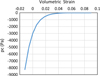 |
Fig. A4 Hardening curve for sand lithology. |
Appendix 2 Material parameters
References
- Albertz M., Lingrey S. (2012) Critical state finite element models of contractional fault-related folding: Part 1. Structural analysis. Tectonophysics 576–577, 133–149. [CrossRef] [Google Scholar]
- Albertz M., Sanz P.F. (2012) Critical state finite element models of contractional fault-related folding: Part 2. Mechanical analysis. Tectonophysics 576–577, 150–170. [CrossRef] [Google Scholar]
- Bernaud D., Dormieux L., Maghous S. (2006) A constitutive and numerical model for mechanical compaction in sedimentary basins. Computers Geotechnics 33, 6–7, 316–329. [CrossRef] [Google Scholar]
- Bolås H.M.N., Hermanrud C., Teige G.M.G. (2004) Origin of overpressures in shales: Constraints from basin modeling. AAPG Bulletin 88, 193–211. [CrossRef] [Google Scholar]
- Boyer S.E., Elliott D. (1982) Thrust systems. AAPG Bulletin 66, 9, 1196–1230. [Google Scholar]
- Butlers R.W.H., Paton D.A. (2010) Evaluating lateral compaction in deepwater fold and thrust belts: How much are we missing from “nature's sandbox”? GSA Today 20, 3, 4–10. [CrossRef] [Google Scholar]
- Chauvin B.P., Lovely P., Stockmeyer J.M., Plesch A., Caumon G., Shaw J.H. (2018) Validating novel boundary conditions for 3D mechanics-based restoration: an extensional sandbox model example. AAPG Bulletin 102, 2, 245–266. [CrossRef] [Google Scholar]
- Crook A.J.L. (2013) ParaGeo: a finite element model for coupled simulation of the evolution of geological structures. Three Cliffs Geomechanical Analysis, Swansea, UK. [Google Scholar]
- Crook A.J.L., Willson S.M., Yu J.G., Owen D.R.J. (2006) Predictive modelling of structure evolution in sandbox experiments. J. Struct. Geol. 28, 5, 729–744. [CrossRef] [Google Scholar]
- Dahlstrom C.D.A. (1969) Balanced cross sections. Can. J. Earth Sci. 6, 743–757. [CrossRef] [Google Scholar]
- Durand-Riard P., Guzofski C., Caumon G., Titeux M. (2012) Handling natural complexity in three-dimensional geomechanical restoration, with application to the recent evolution of the outer fold and thrust belt, deep-water Niger Delta. AAPG Bulletin 97, 1, 87–102. [CrossRef] [Google Scholar]
- Durand-Riard P., Salles L., Ford M., Caumon G., Pellerin J. (2011) Understanding the evolution of syn-depositional folds: Coupling decompaction and 3D sequential restoration. Marine Petroleum Geol. 28, 8, 1530–1539. [CrossRef] [Google Scholar]
- Durand-Riard P., Shaw J.H., Plesch A., Lufadeju G. (2013) Enabling 3D geomechanical restoration of strike- and oblique-slip faults using geological constraints, with applications to the deep-water Niger Delta. J. Struct. Geol. 48, 3, 33–44. [CrossRef] [Google Scholar]
- Estublier A., Fornel A., Brosse E., Houel P., Lecomte J.C., Delmas J., Vincké O. (2017) Simulation of a Potential CO2 Storage in the West Paris Basin: Site Characterization and Assessment of the Long-Term Hydrodynamical and Geochemical Impacts Induced by the CO2 Injection. Oil & Gas Sci. Technol. − Rev. IFP Energies nouvelles 72, 22 [CrossRef] [Google Scholar]
- Faille I., Thibaut M., Cacas M.-C., Havé P., Willien F., Wolf S., Agelas L., Pegaz-Fiornet S. (2014) Modeling fluid flow in faulted basins. Oil & Gas Sci. Technol – Rev. IFP Energies nouvelles 69, 4, 529–553 [CrossRef] [EDP Sciences] [Google Scholar]
- Fujii Y. (2012) Weakness plane model to simulate effects of stress states on rock strengths. True Triaxial Testing of Rocks Workshop, Beijing, China. [Google Scholar]
- Fujii Y., Kodama J., Fukuda D. (2013) 3-D Weakness Plane Model to Clarify the Mechanisms of Influences of Stress States on Rock Strengths. J. Min. Mater. Process. Inst. Jpn. 129, 7, 467–471. [Google Scholar]
- Gibbs A.D. (1983) Balanced cross-section construction from seismic sections in areas of extensional tectonics. J. Struct. Geology 5, 153–160. [Google Scholar]
- Griffiths P.A., Jones S., Salter N., Schaefer F., Osfield R., Reiser H. (2002) Flexural slip unfolding: a new technique for 3-D flexural-slip restoration. J. Struct. Geol. 24, 4, 773–782. [CrossRef] [Google Scholar]
- Gutierrez M., Wangen M. (2005) Modeling of compaction and overpressuring in sedimentary basins. Marine Petrol. Geol. 22, 351–363. [CrossRef] [Google Scholar]
- Guzofski C., Joachim Mueller P, Shaw J.H., Muron P., Medwedeff D.A., Bilotti F., Rivero C. (2009) Insights into the mechanisms of fault-related folding provided by volumetric structural restorations using spatially varying mechanical constraints. AAPG Bulletin 93, 4, 479–502. [CrossRef] [Google Scholar]
- Hantschel T., Kauerauf A.I. (2009) Fundamentals of Basin and Petroleum Systems Modeling. Springer-Verlag, Berlin [Google Scholar]
- Hardy S., Finch E. (2007) Mechanical stratigraphy and the transition from trishear to kink-band fault-propagation fold forms above blind basement thrust faults:a discrete-element study. Marine Petrol. Geol. 24, 75–90. [CrossRef] [Google Scholar]
- Higgins S., Clarke B., Davies R.J., Cartwright J. (2009) Internal geometry and growth history of thrust-related anticline in a deep water fold belt. J. Struct. Geol. 31, 12, 1597–1611. [CrossRef] [Google Scholar]
- Kjeldstad A., Skogseid J., Langtangen H.P., Bjørlykke K., Høeg K. (2003) Differential loading by prograding sedimentary wedges on continental margins: An arch-forming mechanism. J. Geophys. Res. 108, B1, 2036). [Google Scholar]
- Krueger S., Grant N. (2011). The growth history of toe thrusts of the Niger Delta and the role of pore pressure. Thrust fault-related folding: AAPG Memoir. 94, 357–390. [Google Scholar]
- Kusznir N., Roberts A.M., Morley C. K. (1995) Forward and reverse modelling of rift basin formation. Hydrocarbon Habitat in Rift Basins. J. J. Lambiase. London, Geological Society. 80: 33–56. [Google Scholar]
- Lewis R.W., Schrefler B.A. (1998). The finite element method in the static and dynamic deformation and consolidation of porous media, Wiley, Chichester, UK [Google Scholar]
- Lopez-Mir B., Muñoz J.A., García J. (2014) Restoration of basins driven by extension and salt tectonics: Example from the Cotiella Basin in the central Pyrenees. J. Struct. Geol. 69: 147–162. [CrossRef] [Google Scholar]
- Lovely P., Flodin E., Guzofski C., Maerten F., Pollard D.D. (2012) Pitfalls among the promises of mechanics-based restoration: Addressing implications of unphysical boundary conditions. J. Struct. Geol 41, 47–63. [CrossRef] [Google Scholar]
- Luo G., Hudec M.R., Flemings P.B., Nikolinakou M.A. (2017) Deformation, stress and pore pressure in an evolving suprasalt basin. J. Geophys. Res: Solid Earth 122, 7, 5663–5690. [Google Scholar]
- Luo G., Nikolinakou M.A., Flemings P.B., Hudec M.R. (2012) Geomechanical modeling of stresses adjacent to salt bodies: Part 1—Uncoupled models. AAPG Bulletin 96, 1, 43–64. [CrossRef] [Google Scholar]
- Maerten L., Maerten F. (2006) Chronologic modeling of faulted and fractured reservoirs using geomechanically based restoration: technique and industry applications. AAPG Bulletin 90, 8, 1201–1226. [CrossRef] [Google Scholar]
- Maghous S., Brüch A., Bernaud D., Dormieux L., Braun A. L. (2014) Two-dimensionalfinite element analysis of gravitational and lateraldriven deformation in sedimentary basins. Int. J. Numer. Anal. Meth. Geomech. 38, 725–746. [CrossRef] [Google Scholar]
- Moore G.F., Saffer D., Studer M., Costa Pisani P. (2011) Structural restoration of thrusts at the toe of the Nankai Trough accretionary prism off Shikoku Island, Japan: Implications for dewatering processes. Geochem. Geophys. Geosyst. 12, 5, 1–15. [Google Scholar]
- Moretti I., Lepage F., Guiton M. (2006) KINE3D: a new 3D restoration method based on a mixed approach linking geometry and geomechanics. Oil Gas Sci. Technol. 61, 2, 277–289. [CrossRef] [Google Scholar]
- Muron P. (2005) 3-D numerical methods for the restoration of faulted geological structures. Lorraine, France, Institut National Polytechnique de Lorraine: 131. [Google Scholar]
- Nikolinakou M.A., Flemings P.B., Hudec M.R. (2014) Modeling stress evolution around a rising salt diapir. Marine Petrol. Geol. 51, 230–238. [CrossRef] [Google Scholar]
- Nikolinakou M.A., Luo G., Hudec M.R., Flemings P.B. (2012) Geomechanical modeling of stresses adjacent to salt bodies: Part 2—Poroelastoplasticity and coupled overpressures. AAPG Bulletin 96, 1, 65–85. [CrossRef] [Google Scholar]
- Nyantakyi E.K., Tao L., Wangshui H., Borkloe J.K. (2014) The role of geomechanical-based structural restoration in reservoir analysis of deepwater Niger Delta, Nigeria. Acta Geodaetica et Geophysica 49, 4, 415–429. [CrossRef] [Google Scholar]
- Nygård R., Gutierrez M., Bratli R.K., Høeg K. (2006) Brittle-ductile transition, shear failure and leakage in shales and mudrocks. Marine Petrol. Geol. 23, 2, 201–212. [CrossRef] [Google Scholar]
- Nygård R., Gutierrez M., Gautam R., Høeg K. (2004a) Compaction behaviour of argillaceous sediments as function of diagenesis. Marine Petrol. Geol. 21, 349–362. [CrossRef] [Google Scholar]
- Nygård R., Gutierrez M., Høeg K., Bjørlykke K. (2004b) Influence of burial history on microstructure and compaction behaviour of Kimmeridge clay. Petroleum Geoscience 10, 3, 259–270. [CrossRef] [Google Scholar]
- Obradors-Prats J., Rouainia M., Aplin A.C., Crook A.J.L. (2016) Stress and pore pressure in complex tectonic settings predicted with coupled, 3D geomechanical-fluid flow models. Marine Petrol. Geol. 76, 9, 464–477. [CrossRef] [Google Scholar]
- Obradors-Prats J., Rouainia M., Aplin A.C., Crook A.J.L. (2017a) Assessing the implications of tectonic compaction on pore pressure using a coupled geomechanical approach. Marine Petroleum Geol. 79, 1, 31–43. [CrossRef] [Google Scholar]
- Obradors-Prats J., Rouainia M., Aplin A.C., Crook A.J.L. (2017b) Hydromechanical Modeling of Stress, Pore Pressure, and Porosity Evolution in Fold-and-Thrust Belt Systems. J. Geophys. Res: Solid Earth 122, 11, 9383–9403. [CrossRef] [Google Scholar]
- Peric D., Crook A.J.L. (2004) Computational strategies for predictive geology with reference to salt tectonics. Comput. Methods Appl. Mech. Eng. 193, 48–51, 5195–5222. [CrossRef] [Google Scholar]
- Roberts D.T., Crook A.J.L., Profit M.L., Cartwright J.A. (2015). Investigating the Evolution of Polygonal Fault Systems Using Geomechanical Forward Modeling. 49th US Rock Mechanics/Geomechanics Symposium. San Francisco, CA, USA, ARMA. [Google Scholar]
- Rowan M.G., Kligfield R. (1989) Cross-section restoration and balancing as an aid to seismic interpretation in extensional terrains. AAPG Bulletin 73, 955–966. [Google Scholar]
- Rowan M.G., Ratliff R.A. (2012) Cross-section restoration of salt-related deformation: Best practices and potential pitfalls. J. Struct. Geol. 41, 8, 24–37. [CrossRef] [Google Scholar]
- Ruh J.B. (2017) Effect of fluid pressure distribution on the structural evolution of acretionary wedges. Terra Nova 29, 202–210. [CrossRef] [Google Scholar]
- Schneider F., Potdevin J.L., Wolf S., Faille I. (1996) Mechanical and chemical compaction model for sedimentary basin simulators. Tectonophysics 263, 1–4, 307–317. [CrossRef] [Google Scholar]
- Smart K.J., Ferrill D.A., Morris A.P., McGinnis R.N. (2012) Geomechanical modeling of stress and strain evolution during contractional fault-related folding. Tectonophysics 171–196. [CrossRef] [Google Scholar]
- Spinelli G.A., Mozley P.S., Tobin H.J., Underwood M.B., Hoffman N. W., Bellew G.M. (2007) Diagenesis, sediment strength, and pore collapse in sediment approaching the Nankai Trough subduction zone. GSA Bulletin 119, 3/4, 377–390. [CrossRef] [Google Scholar]
- Thibaut M., Jardin A., Faille I., Willien F., Guichet X. (2014) Advanced Workflows for Fluid Transfer in Faulted Basins. Oil & Gas Sci. Technol − Rev. IFP Energies nouvelles 69, 4, 573–584. [CrossRef] [Google Scholar]
- Thornton D.A., Crook A.J.L. (2014) Predictive modelling of the evolution of fault structure: 3-D modelling and coupled geomechanical/flow simulation. Rock Mech. Rock Eng. 47, 5, 1533–1549. [CrossRef] [Google Scholar]
- Welch M.J., Knipe R.J., Souque C., Davies R.K. (2009) A Quadshear kinematic model for folding and clay smear development in fault zones. Tectonophysics 471, 3–4, 186–202. [CrossRef] [Google Scholar]
- Woillez M.N., Souque C., Rudkiewicz J.L., Willien F., Cornu T. (2017) Insights in Fault Flow Behaviour from Onshore Nigeria Petroleum System Modelling. Oil & Gas Sci. Technol − Rev. IFP Energies nouvelles 72 31. [Google Scholar]
- White S.H., Bretan P.G., Rutter E.H. (1986) Fault-Zone reactivation: kinematics and mechanisms. Philosophical Transactions of the Royal Society of London. Series A, Math. Phys. Sci. 317, 1539, 81–97 [CrossRef] [Google Scholar]
- Wood D.M. (1990) Soil Behaviour and Critical State Soil Mechanics, Cambridge University Press, Cambridge, UK [Google Scholar]
All Tables
All Figures
|
Fig. 1 Schematic example of the boundary conditions adopted for back striping the top surface to a restoration surface. (a) Initial geometry configuration (present day), (b) restored geometry configuration. |
| In the text | |
|
Fig. 2 Schematic representation of several restoration options available in ParaGeo. (a) Isotropic elasticity, (b) transverse isotropic elasticity, (c) distributed intra-layer bedding plane slip model and (d) inter-layer bedding plane slip using contact surfaces. |
| In the text | |
|
Fig. 3 Flowcharts for improving restorations following an integrated workflow of restoration and forward simulation. |
| In the text | |
|
Fig. 4 Restoration sequence from present day to restoration step 3. The red curve indicates the tracked geometry horizon that will define the boundary conditions for the forward simulation. |
| In the text | |
|
Fig. 5 Forward simulation prescribed basal boundary shape evolution derived from restoration. |
| In the text | |
|
Fig. 6 Comparison of final configuration geometries and plastic strain contours for the Target model (a) and (c) and the restoration-derived forward simulation (b) and (d). |
| In the text | |
|
Fig. 7 Examples of the two fault triggering methods, fault insertion (a), (c) and fault seeding (b) and (d). Figures (a) and (b) show undeformed geometries with the initial conditions at fault location. Note that the fault path in (a) is used to split the continuous geometry at early stages of the simulation. Figures (c) and (d) show the model mesh after the first deformational stage of the simulation. |
| In the text | |
|
Fig. 8 Schematic model initial geometry showing the location of the seeded faults. |
| In the text | |
|
Fig. 9 Predicted geometry (a) and plastic strain contours (b) at the upper edge of the model after deposition of five layers for the case with fault seeding. |
| In the text | |
|
Fig. 10 (a) Restoration model for an isolated thrust structure from Niger Delta. The geometry has been obtained from Higgins et al. (2009). The horizons are numbered consistently with the reference; i.e. h1 for the model base to h11 for the top surface. Note that intra-formation fault tips have been neglected. (b) Prescribed initial porosity distribution with depth. This porosity distribution is representative of Niger Delta sediments and has been obtained from the field data published by Krueger and Grant (2011). (c) Final restored geometry after restoration of 8 formations. |
| In the text | |
|
Fig. 11 (a) Comparison of the field geometry, (b) with restoration-derived forward simulations predictions for cases using fault insertion algorithm, using fault insertion algorithm, (c) incorporating correction in the shortening and (d) without fault insertion but including correction in the shortening. |
| In the text | |
|
Fig. 12 Horizontal strain distribution in the predicted structure. Negative values stand for compressive strains whereas positive values stand for extensional strain. |
| In the text | |
|
Fig. A1 Initial geometry and boundary conditions for the Target model (not drawn to scale). |
| In the text | |
|
Fig. A2 Evolution of Target model geometry. Colours indicate the different formations. |
| In the text | |
|
Fig. A3 (a) Plastic strain contours at final configuration. The maximum plastic strain has been limited to 5 so all the strain localizations are visible but the maximum plastic strain value reached 50 (Plastic strain of 1 corresponds to 100% of strain), (b) Material grid showing the deformation structures. Major synthetic and antithetic faults are highlighted with white and black curves respectively. |
| In the text | |
|
Fig. A4 Hardening curve for sand lithology. |
| In the text | |